SAS and R

Reader Annisa Mike asked in a comment on an early post about power calculation for logistic regression with an interaction.

This is a topic that has come up with increasing frequency in grant proposals and article submissions. We'll begin by showing how to simulate data with the interaction, and in our next post we'll show how to assess power to detect the interaction using simulation.

As in our earlier post, our method is to construct the linear predictor and the link function separately. This should help to clarify the roles of the parameter values and the simulated data.

SAS
In keeping with Annisa Mike's question, we'll simulate the interaction between a categorical and a continuous covariate. We'll make the categorical covariate dichotomous and the continuous one normal. To keep things simple, we'll leave the main effects null-- that is, the effect of the continuous covariate when the dichotomous one is 0 is also 0.

data test;
do i = 1 to 1000;
 c = (i gt 500);
 x = normal(0);
 lp = -3 + 2*c*x;
 link_lp = exp(lp)/(1 + exp(lp));
 y = (uniform(0) lt link_lp); 
 output;
end;
run;

In proc logistic, unlike other many other procedures, the default parameterization for categorical predictors is effect cell coding. This can lead to unexpected and confusing results. To get reference cell coding, use the syntax for the class statement shown below. This is similar to the default result for the glm procedure. If you need identical behavior to the glm procedure, use param = glm. The desc option re-orders the categories to use the smallest value as the reference category.

proc logistic data = test plots(only)=effect(clband);
class c (param = ref desc);
model y(event='1') = x|c;
run;

The plots(only)=effect(clband) construction in the proc logistic statement generates the plot shown above. If c=0, the probability y=1 is small for any value of x, and a slope of 0 for x is tenable. If c=1, the probability y=1 increases as x increases and nears 1 for large values of x.

The parameters estimated from the data show good fidelity to the selected values, though this is merely good fortune-- we'd expect the estimates to often be more different than this.

 Standard Wald
Parameter DF Estimate Error Chi-Square Pr> ChiSq
Intercept 1 -3.0258 0.2168 194.7353 <.0001 x 1 -0.2618 0.2106 1.5459 0.2137 c 1 1 -0.0134 0.3387 0.0016 0.9685 x*c 1 1 2.0328 0.3168 41.1850 <.0001 

R
As sometimes occurs, the R code resembles the SAS code. Creating the data, in fact, is quite similar. The main differences are in the names of the functions that generate the randomness and the vectorized syntax that avoids the looping of the SAS datastep.

c = rep(0:1,each=500)
x = rnorm(1000)
lp = -3 + 2*c*x
link_lp = exp(lp)/(1 + exp(lp))
y = (runif(1000) < link_lp) 

We fit the logistic regression with the glm() function, and examine the parameter estimates.

log.int = glm(y~as.factor(c)*x, family=binomial)
summary(log.int)

Here, the estimate for the interaction term is further from the selected value than we lucked into with the SAS simulation, but the truth is well within any reasonable confidence limit.

 Estimate Std. Error z value Pr(>|z|) 
(Intercept) -3.3057 0.2443 -13.530 < 2e-16 *** as.factor(c)1 0.4102 0.3502 1.171 0.241 x 0.2259 0.2560 0.883 0.377 as.factor(c)1:x 1.7339 0.3507 4.944 7.66e-07 *** 

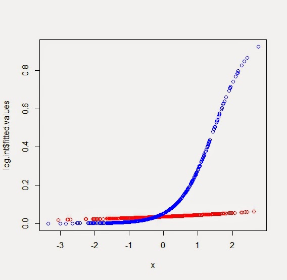
A simple plot of the predicted values can be made fairly easily. The predicted probabilities of y=1 reside in the summary object as log.int$fitted.values. We can color them according to the values of the categorical predictor by defining a color vector and then choosing a value from the vector for each observation. The resulting plot is shown below. If we wanted confidence bands as in the SAS example, we could get standard error for the (logit scale) predicted values using the predict() function with the se.fit option.

mycols = c("red","blue")
plot(log.int$fitted.values ~ x, col=mycols[c+1])

An unrelated note about aggregators: We love aggregators! Aggregators collect blogs that have similar coverage for the convenience of readers, and for blog authors they offer a way to reach new audiences. SAS and R is aggregated by R-bloggers, PROC-X, and statsblogs with our permission, and by at least 2 other aggregating services which have never contacted us. If you read this on an aggregator that does not credit the blogs it incorporates, please come visit us at SAS and R. We answer comments there and offer direct subscriptions if you like our content. In addition, no one is allowed to profit by this work under our license; if you see advertisements on this page, the aggregator is violating the terms by which we publish our work.

A colleague recently contacted us with the following question: "My outcome is skewed-- how can I compare medians across multiple categories?"

What they were asking for was a generalization of the Wilcoxon rank-sum test (also known as the Mann-Whitney-Wilcoxon test, among other monikers) to more than two groups. For the record, the answer is that the Kruskal-Wallis test is the generalization of the Wilcoxon, the one-way ANOVA to the Wilcoxon's t-test.

But this question is based on a false premise: that the the Wilcoxon rank-sum test is used to compare medians. The premise is based on a misunderstanding of the null hypothesis of the test. The actual null hypothesis is that there is a 50% probability that a random value from one population exceeds an random value from the other population. The practical value of this is hard to see, and thus in many places, including textbooks, the null hypothesis is presented as "the two populations have equal medians". The actual null hypothesis can be expressed as the latter median hypothesis, but only under the additional assumption that the shapes of the distributions are identical in each group.

In other words, our interpretation of the test as comparing the medians of the distributions requires the location-shift-only alternative to be the case. Since this is rarely true, and never assessed, we should probably use extreme caution in using, and especially in interpreting, the Wilcoxon rank-sum test.

To demonstrate this issue, we present a simple simulation, showing a case of two samples with equal medians but very different shapes. In one group, the values are exponential with mean = 1 and therefore median log 2, in the other they are normal with mean and median = log 2 and variance = 1. We generate 10,000 observations and show that the Wilcoxon rank-sum test rejects the null hypothesis. If we interpret the null incorrectly as applying to the medians, we will be misled. If our interest actually centered on the medians for some reasons, an appropriate test that would not be sensitive to the shape of the distribution could be found in a quantile regression. Another, of course, would be the median test. We show that this test does not reject the null hypothesis of equal medians, even with the large sample size.

We leave aside the deeper questions of whether comparing medians is a useful substitute for comparing means, or whether means should not be compared when distributions are skewed.

R
In R, we simulate two separate vectors of data, then feed them directly to the wilcox.test() function (section 2.4.2).

y1 = rexp(10000)
y2 = rnorm(10000) + log(2)
wilcox.test(y1,y2)

This shows a very small p-value, denoting the fact not that the medians are unequal but that one or the other of these distributions generally has larger values. Hint: it might be the one with the long tail and no negative values.

 Wilcoxon rank sum test with continuity correction
data: y1 and y2
W = 55318328, p-value < 2.2e-16 alternative hypothesis: true location shift is not equal to 0 

To set up the quantile regression, we put the observations into a single vector and make a group indicator vector. Then we load the quantreg package and use the rq() function (section 4.4.4) to fit the median regression.

y = c(y1,y2)
c = rep(1:2, each = 10000)
library(quantreg)
summary(rq(y~as.factor(c)))

This shows we would fail to reject the null of equal medians.

Call: rq(formula = y ~ as.factor(c))
tau: [1] 0.5
Coefficients:
 Value Std. Error t value Pr(>|t|)
(Intercept) 0.68840 0.01067 64.53047 0.00000
as.factor(c)2 -0.00167 0.01692 -0.09844 0.92159
Warning message:
In rq.fit.br(c, y, tau = tau, ...) : Solution may be nonunique

SAS
In SAS, we make a data set with a group indicator and use it to generate data conditionally.

data wtest;
do i = 1 to 20000;
 c = (i gt 10000);
 if c eq 0 then y = ranexp(0);
 else y = normal(0) + log(2);
 output;
 end;
run;

The Wilcoxon rank-sum test is in proc npar1way (section 2.4.2).

proc npar1way data = wtest wilcoxon;
class c;
var y;
run;

As with R, we find a very small p-value.

 The NPAR1WAY Procedure
 Wilcoxon Scores (Rank Sums) for Variable y
 Classified by Variable c
 Sum of Expected Std Dev Mean
 c N Scores Under H0 Under H0 Score
 0 10000 106061416 100005000 408258.497 10606.1416
 1 10000 93948584 100005000 408258.497 9394.8584
 Wilcoxon Two-Sample Test
 Statistic 106061416.0000
 Normal Approximation
 Z 14.8348
 One-Sided Pr> Z <.0001 Two-Sided Pr> |Z| <.0001 t Approximation One-Sided Pr> Z <.0001 Two-Sided Pr> |Z| <.0001 Z includes a continuity correction of 0.5. Kruskal-Wallis Test Chi-Square 220.0700 DF 1 Pr> Chi-Square <.0001 

The median regression is in proc quantreg (section 4.4.4). As in R, we fail to reject the null of equal medians.

proc quantreg data =wtest;
class c;
model y = c;
run;

 The QUANTREG Procedure
 Quantile and Objective Function
 Predicted Value at Mean 0.6909
 Parameter Estimates
 Standard 95% Confidence
 Parameter DF Estimate Error Limits t Value
 Intercept 1 0.6909 0.0125 0.6663 0.7155 55.06
 c 0 1 0.0165 0.0160 -0.0148 0.0479 1.03
 c 1 0 0.0000 0.0000 0.0000 0.0000 .
 Parameter Estimates
 Parameter Pr> |t|
 Intercept <.0001 c 0 0.3016 c 1 . 

An unrelated note about aggregators: We love aggregators! Aggregators collect blogs that have similar coverage for the convenience of readers, and for blog authors they offer a way to reach new audiences. SAS and R is aggregated by R-bloggers, PROC-X, and statsblogs with our permission, and by at least 2 other aggregating services which have never contacted us. If you read this on an aggregator that does not credit the blogs it incorporates, please come visit us at SAS and R. We answer comments there and offer direct subscriptions if you like our content. In addition, no one is allowed to profit by this work under our license; if you see advertisements on this page, the aggregator is violating the terms by which we publish our work.

Shared frailty models are a way of allowing correlated observations into proportional hazards models. Briefly, instead of l_i(t) = l_0(t)e^(x_iB), we allow l_ij(t) = l_0(t)e^(x_ijB + g_i), where observations j are in clusters i, g_i is typically normal with mean 0, and g_i is uncorrelated with g_i'. The nomenclature frailty comes from examining the logs of the g_i and rewriting the model as l_ij(t) = l_0(t)u_i*e^(xB) where the u_i are now lognormal with median 0. Observations j within cluster i share the frailty u_i, and fail faster (are frailer) than average if u_i> 1.

In SAS 9.2, this model could not be fit, though it is included in the survival package in R. (Section 4.3.2) With SAS 9.3, it can now be fit. We explore here through simulation, extending the approach shown in example 7.30.

SAS
To include frailties in the model, we loop across the clusters to first generate the frailties, then insert the loop from example 7.30, which now represents the observations within cluster, adding the frailty to the survival time model. There's no need to adjust the censoring time.

data simfrail;
 beta1 = 2;
 beta2 = -1;
 lambdat = 0.002; *baseline hazard;
 lambdac = 0.004; *censoring hazard;
 do i = 1 to 250; *new frailty loop;
 frailty = normal(1999) * sqrt(.5);
 do j = 1 to 5; *original loop;
 x1 = normal(0);
 x2 = normal(0);
 * new model of event time, with frailty added;
 linpred = exp(-beta1*x1 - beta2*x2 + frailty);
 t = rand("WEIBULL", 1, lambdaT * linpred);
 * time of event;
 c = rand("WEIBULL", 1, lambdaC);
 * time of censoring;
 time = min(t, c); * which came first?;
 censored = (c lt t);
 output;
 end;
 end;
run;

For comparison's sake, we replicate the naive model assuming independence:

proc phreg data=simfrail;
 model time*censored(1) = x1 x2;
run;

 Parameter Standard Hazard
 Parameter DF Estimate Error Chi-Square Pr> ChiSq Ratio

 x1 1 1.68211 0.05859 824.1463 <.0001 5.377
 x2 1 -0.88585 0.04388 407.4942 <.0001 0.412

The parameter estimates are rather biased. In contrast, here is the correct frailty model.

proc phreg data=simfrail;
 class i;
 model time*censored(1) = x1 x2;
 random i / noclprint;
run;
 Cov REML Standard
 Parm Estimate Error

 i 0.5329 0.07995

 Parameter Standard Hazard
 Parameter DF Estimate Error Chi-Square Pr> ChiSq Ratio

 x1 1 2.03324 0.06965 852.2179 <.0001 7.639
 x2 1 -1.00966 0.05071 396.4935 <.0001 0.364

This returns estimates gratifyingly close to the truth. The syntax of the random statement is fairly straightforward-- the noclprint option prevents printing all the values of i. The clustering variable must be specified in the class statement. The output shows the estimated variance of the g_i.

R
In our book (section 4.16.14) we show an example of fitting the uncorrelated data model, but we don't display a frailty model. Here, we use the data generated in SAS, so we omit the data simulation in R. As in SAS, it would be a trivial extension of the code presented in example 7.30. For parallelism, we show the results of ignoring the correlation, first.

> library(survival)
> with(simfrail, coxph(formula = Surv(time, 1-censored) ~ x1 + x2))

 coef exp(coef) se(coef) z p
x1 1.682 5.378 0.0586 28.7 0
x2 -0.886 0.412 0.0439 -20.2 0

with identical results to above. Note that the Surv function expects an indicator of the event, vs. SAS expecting a censoring indicator.

As with SAS, the syntax for incorporating the frailty is simple.

> with(simfrail, coxph(formula = Surv(time, 1-censored) ~ x1 + x2 
 + frailty(i)))

 coef se(coef) se2 Chisq DF p
x1 2.02 0.0692 0.0662 850 1 0
x2 -1.00 0.0506 0.0484 393 1 0
frailty(i) 332 141 0

Variance of random effect= 0.436

Here, the results differ slightly from the SAS model, but still return parameter estimates that are quite similar. We're not familiar enough with the computational methods to diagnose the differences.

To simulate survival data with censoring, we need to model the hazard functions for both time to event and time to censoring.

We simulate both event times from a Weibull distribution with a scale parameter of 1 (this is equivalent to an exponential random variable). The event time has a Weibull shape parameter of 0.002 times a linear predictor, while the censoring time has a Weibull shape parameter of 0.004. A scale of 1 implies a constant (exponential) baseline hazard, but this can be modified by specifying other scale parameters for the Weibull random variables.

First we'll simulate the data, then we'll fit a Cox proportional hazards regression model (section 4.3.1) to see the results.

Simulation is relatively straightforward, and is helpful in concretizing the notation often used in discussion survival data. After setting some parameters, we generate some covariate values, then simply draw an event time and a censoring time. The minimum of these is "observed" and we record whether it was the event time or the censoring time.

SAS

data simcox;
 beta1 = 2;
 beta2 = -1;
 lambdat = 0.002; *baseline hazard;
 lambdac = 0.004; *censoring hazard;
 do i = 1 to 10000;
 x1 = normal(0);
 x2 = normal(0);
 linpred = exp(-beta1*x1 - beta2*x2);
 t = rand("WEIBULL", 1, lambdaT * linpred);
 * time of event;
 c = rand("WEIBULL", 1, lambdaC);
 * time of censoring;
 time = min(t, c); * which came first?;
 censored = (c lt t);
 output;
 end;
run;

The phreg procedure (section 4.3.1) will show us the effects of the censoring as well as the results of fitting the regression model. We use the ODS system to reduce the output.

ods select censoredsummary parameterestimates;
proc phreg data=simcox;
 model time*censored(1) = x1 x2;
run;

The PHREG Procedure

Summary of the Number of Event and Censored Values
 
 Percent
 Total Event Censored Censored
 10000 5971 4029 40.29

 Analysis of Maximum Likelihood Estimates
 
 Parameter Standard
Parameter DF Estimate Error Chi-Square Pr> ChiSq

x1 1 1.98628 0.02213 8059.0716 <.0001
x2 1 -1.01310 0.01583 4098.0277 <.0001

Analysis of Maximum Likelihood Estimates
 
 Hazard
Parameter Ratio

x1 7.288
x2 0.363

R

n = 10000
beta1 = 2; beta2 = -1
lambdaT = .002 # baseline hazard
lambdaC = .004 # hazard of censoring

x1 = rnorm(n,0)
x2 = rnorm(n,0)
# true event time
T = rweibull(n, shape=1, scale=lambdaT*exp(-beta1*x1-beta2*x2)) 
C = rweibull(n, shape=1, scale=lambdaC) #censoring time
time = pmin(T,C) #observed time is min of censored and true
event = time==T # set to 1 if event is observed

Having generated the data, we assess the effects of censoring with the table() function (section 2.2.1) and load the survival() library to fit the Cox model.

> table(event)
event
FALSE TRUE 
 4083 5917 

> library(survival)
> coxph(Surv(time, event)~ x1 + x2, method="breslow")
Call:
coxph(formula = Surv(time, event) ~ x1 + x2, method = "breslow")


 coef exp(coef) se(coef) z p
x1 1.98 7.236 0.0222 89.2 0
x2 -1.02 0.359 0.0160 -64.2 0

Likelihood ratio test=11369 on 2 df, p=0 n= 10000 

These parameters result in data where approximately 40% of the observations are censored. The parameter estimates are similar to the true parameter values.

In example 7.20, we showed how to simulate categorical data. But we might anticipate needing to do that frequently. If a SAS function weren't built in and an equivalent R function not available in a package, we could build them from scratch.

SAS

The SAS code is particularly tortured, since we must parse the parameter string to extract the table probabilities. We do this with the count and find (section 1.4.6) and substr (section 1.4.3) functions. We also turn the characters into numbers (section 1.4.2). The SAS Macro (section A.8.1) runs a data step, so it cannot be called from within another data step, as would usually be desirable. Instead, you would have to generate the data and then merge it into any additional data that was required. On the whole, it might make more sense to treat every application as a special case and hand-code each one, rather than to use the macro, were a built-in function not available.

%macro rtable(outdata=, outvar=, n=1, p=);
data &outdata (keep=&outvar);
/* In the first section of code, we determine the number
 of categories and set up an array to hold the 
 probabilities for each category. A maximum number of 
 catagories must be provided; here we use 100. */
nprobs = count(&p,",");
lengthprobs = length(&p);
array probs [100] _temporary_;

/* In the next section we parse the parameter string to 
 extract the probabilities for each category. */
lastcomma = 0;
lastprob = 0;
do prob = 1 to nprobs;
 nextcomma = find(&p,",",lastcomma +1);
 probs[prob] = lastprob + 
 substr(&p,lastcomma+1, (nextcomma-lastcomma -1));
 lastcomma = nextcomma;
 lastprob = probs[prob];
 end;
/* Finally, we generate a uniform random variate and
 use it to find the appropriate category. */
do i = 1 to &n;
 __x = uniform(0);
 &outvar = 1;
 do j = 1 to nprobs;
 &outvar = &outvar + (__x gt probs[j]);
 end;
 output;
 end;
run;
%mend rtable;

We've left this code so that an extra comma must be included in the probability parameter string. This could be fixed with an additional line or two in the data step.

We can then run the macro and test the resulting data using proc freq.

%rtable(outdata=test2,outvar= mycat, n = 10000, 
 p = ".1,.2,.3,");

proc freq data = test2; tables mycat; run;

 Cumulative Cumulative
mycat Frequency Percent Frequency Percent
------------------------------------------------------
 1 1032 10.32 1032 10.32
 2 2013 20.13 3045 30.45
 3 2956 29.56 6001 60.01
 4 3999 39.99 10000 100.00

R

In contrast, the R code to write a function (section B.5.2) is trivial, using the cut() function as suggested by Douglas Rivers, discussed in section 1.4.10.

rtable1 <- function(cuts,n) {
 output <- cut(runif(n), cuts, labels=FALSE)
 return(output)
}

In fact, the function hardly seems worth writing. To use it, you need to include 0 and 1 as the first and last elements of the cuts vector. Results can be examined using the table() function (section 2.2.1)

> mycat1 <- rtable1(c(0,.1,.3,.6,1),10000)
> summary(factor(mycat1))
 1 2 3 4 
1058 1989 2978 3975 

To add a little bit of programming to it, suppose we want to list the probabilities per category, rather than the cutpoints. We'll omit the final category probability, assuming the input vector sums to less than 1 and has 1 fewer elements than the desired number of categories.

rtable2 <- function(p, n) {
 cuts <- numeric(length(p) + 2)
 cuts[1] <- 0
 cuts[length(p) + 2] <- 1
 for (k in 1:length(p)) {
 cuts[k+1] <- sum(p[1:k])
 }
 output <- cut(runif(n), cuts, labels=FALSE)
 return(output)
}

The results are similar to the simpler function. We can see the results tabulated without explicitly making the result a factor by using the table() function (section 2.2).

> mycat2 <- rtable2(c(.1, .2, .3), 10000)
> table(mycat2)
mycat2
 1 2 3 4 
 961 1986 3058 3995 

Both SAS and R provide means of simulating categorical data (see section 1.10.4). Alternatively, it is trivial to write code to do this directly. In this entry, we show how to do it once. In a future entry, we'll demonstrate writing a SAS Macro (section A.8.1) and a function in R (section B.5.2) to do it repeatedly.

SAS

data test;
p1 = .1; p2 = .2; p3 = .3;
do i = 1 to 10000;
 x = uniform(0);
 mycat = (x ge 0) + (x gt p1) + (x gt p1 + p2) 
 + (x gt p1 + p2 + p3);
 output;
 end;
run;

Here the parenthetical logical tests in the mycat = line resolve to 1 if the test is true and 0 otherwise, as discussed in section 1.4.9.
The (x ge 0) makes the categories range from 1 to 4, rather than 0 to 3.

The results can be assessed using proc freq:

proc freq data=test; tables mycat; run;

 Cumulative Cumulative
mycat Frequency Percent Frequency Percent
----------------------------------------------------------
 1 947 9.47 947 9.47
 2 2061 20.61 3008 30.08
 3 3039 30.39 6047 60.47
 4 3953 39.53 10000 100.00

R

In contrast, the R syntax to get the results is rather dense.

p <- c(.1,.2,.3)
x <- runif(10000)
mycat <- numeric(10000)
for (i in 0:length(p)) { 
 mycat <- mycat + (x>= sum(p[0:i])) 
 }

We can display the results using the summary() function.

summary(factor(mycat))
 1 2 3 4
 990 2047 2978 3985