SAS and R

Reader Annisa Mike asked in a comment on an early post about power calculation for logistic regression with an interaction.

This is a topic that has come up with increasing frequency in grant proposals and article submissions. We'll begin by showing how to simulate data with the interaction, and in our next post we'll show how to assess power to detect the interaction using simulation.

As in our earlier post, our method is to construct the linear predictor and the link function separately. This should help to clarify the roles of the parameter values and the simulated data.

SAS
In keeping with Annisa Mike's question, we'll simulate the interaction between a categorical and a continuous covariate. We'll make the categorical covariate dichotomous and the continuous one normal. To keep things simple, we'll leave the main effects null-- that is, the effect of the continuous covariate when the dichotomous one is 0 is also 0.

data test;
do i = 1 to 1000;
 c = (i gt 500);
 x = normal(0);
 lp = -3 + 2*c*x;
 link_lp = exp(lp)/(1 + exp(lp));
 y = (uniform(0) lt link_lp); 
 output;
end;
run;

In proc logistic, unlike other many other procedures, the default parameterization for categorical predictors is effect cell coding. This can lead to unexpected and confusing results. To get reference cell coding, use the syntax for the class statement shown below. This is similar to the default result for the glm procedure. If you need identical behavior to the glm procedure, use param = glm. The desc option re-orders the categories to use the smallest value as the reference category.

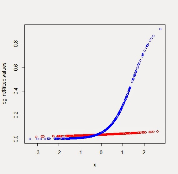
proc logistic data = test plots(only)=effect(clband);
class c (param = ref desc);
model y(event='1') = x|c;
run;

The plots(only)=effect(clband) construction in the proc logistic statement generates the plot shown above. If c=0, the probability y=1 is small for any value of x, and a slope of 0 for x is tenable. If c=1, the probability y=1 increases as x increases and nears 1 for large values of x.

The parameters estimated from the data show good fidelity to the selected values, though this is merely good fortune-- we'd expect the estimates to often be more different than this.

 Standard Wald
Parameter DF Estimate Error Chi-Square Pr> ChiSq
Intercept 1 -3.0258 0.2168 194.7353 <.0001 x 1 -0.2618 0.2106 1.5459 0.2137 c 1 1 -0.0134 0.3387 0.0016 0.9685 x*c 1 1 2.0328 0.3168 41.1850 <.0001 

R
As sometimes occurs, the R code resembles the SAS code. Creating the data, in fact, is quite similar. The main differences are in the names of the functions that generate the randomness and the vectorized syntax that avoids the looping of the SAS datastep.

c = rep(0:1,each=500)
x = rnorm(1000)
lp = -3 + 2*c*x
link_lp = exp(lp)/(1 + exp(lp))
y = (runif(1000) < link_lp) 

We fit the logistic regression with the glm() function, and examine the parameter estimates.

log.int = glm(y~as.factor(c)*x, family=binomial)
summary(log.int)

Here, the estimate for the interaction term is further from the selected value than we lucked into with the SAS simulation, but the truth is well within any reasonable confidence limit.

 Estimate Std. Error z value Pr(>|z|) 
(Intercept) -3.3057 0.2443 -13.530 < 2e-16 *** as.factor(c)1 0.4102 0.3502 1.171 0.241 x 0.2259 0.2560 0.883 0.377 as.factor(c)1:x 1.7339 0.3507 4.944 7.66e-07 *** 

A simple plot of the predicted values can be made fairly easily. The predicted probabilities of y=1 reside in the summary object as log.int$fitted.values. We can color them according to the values of the categorical predictor by defining a color vector and then choosing a value from the vector for each observation. The resulting plot is shown below. If we wanted confidence bands as in the SAS example, we could get standard error for the (logit scale) predicted values using the predict() function with the se.fit option.

mycols = c("red","blue")
plot(log.int$fitted.values ~ x, col=mycols[c+1])

An unrelated note about aggregators: We love aggregators! Aggregators collect blogs that have similar coverage for the convenience of readers, and for blog authors they offer a way to reach new audiences. SAS and R is aggregated by R-bloggers, PROC-X, and statsblogs with our permission, and by at least 2 other aggregating services which have never contacted us. If you read this on an aggregator that does not credit the blogs it incorporates, please come visit us at SAS and R. We answer comments there and offer direct subscriptions if you like our content. In addition, no one is allowed to profit by this work under our license; if you see advertisements on this page, the aggregator is violating the terms by which we publish our work.

Recently a student asked about the difference between confint() and confint.default() functions, both available in the MASS library to calculate confidence intervals from logistic regression models. The following example demonstrates that they yield different results.

R

ds = read.csv("http://www.math.smith.edu/r/data/help.csv")
library(MASS)
glmmod = glm(homeless ~ age + female, binomial, data=ds)

> summary(glmmod)
Call:
glm(formula = homeless ~ age + female, family = binomial, data = ds)

Deviance Residuals: 
 Min 1Q Median 3Q Max 
-1.3600 -1.1231 -0.9185 1.2020 1.5466 

Coefficients:
 Estimate Std. Error z value Pr(>|z|) 
(Intercept) -0.89262 0.45366 -1.968 0.0491 *
age 0.02386 0.01242 1.921 0.0548 .
female -0.49198 0.22822 -2.156 0.0311 *
---
Signif. codes: 0 ‘***’ 0.001 ‘**’ 0.01 ‘*’ 0.05 ‘.’ 0.1 ‘ ’ 1 

(Dispersion parameter for binomial family taken to be 1)

 Null deviance: 625.28 on 452 degrees of freedom
Residual deviance: 617.19 on 450 degrees of freedom
AIC: 623.19

Number of Fisher Scoring iterations: 4

> exp(confint(glmmod))
Waiting for profiling to be done...
 2.5 % 97.5 %
(Intercept) 0.1669932 0.9920023
age 0.9996431 1.0496390
female 0.3885283 0.9522567
> library(MASS)
> exp(confint.default(glmmod))
 2.5 % 97.5 %
(Intercept) 0.1683396 0.9965331
age 0.9995114 1.0493877
female 0.3909104 0.9563045

Why are they different? Which one is correct?

SAS

Fortunately the detailed documentation in SAS can help resolve this. The logistic procedure (section 4.1.1) offers the clodds option to the model statement. Setting this option to both produces two sets of CL, based on the Wald test and on the profile-likelihood approach. (Venzon, D. J. and Moolgavkar, S. H. (1988), “A Method for Computing Profile-Likelihood Based Confidence Intervals,” Applied Statistics, 37, 87–94.)

ods output cloddswald = waldcl cloddspl = plcl;
proc logistic data = "c:\book\help.sas7bdat" plots=none;
class female (param=ref ref='0');
model homeless(event='1') = age female / clodds = both;
run;

 Odds Ratio Estimates and Profile-Likelihood Confidence Intervals

 Effect Unit Estimate 95% Confidence Limits

 AGE 1.0000 1.024 1.000 1.050
 FEMALE 1 vs 0 1.0000 0.611 0.389 0.952


 Odds Ratio Estimates and Wald Confidence Intervals

 Effect Unit Estimate 95% Confidence Limits

 AGE 1.0000 1.024 1.000 1.049
 FEMALE 1 vs 0 1.0000 0.611 0.391 0.956

Unfortunately, the default precision of the printout isn't quite sufficient to identify whether this distinction aligns with the differences seen in the two R methods. We get around this by using the ODS system to save the output as data sets (section A.7.1). Then we can print the data sets, removing the default rounding formats to find all of the available precision.

title "Wald CL";
proc print data=waldcl; format _all_; run;
title "PL CL";
proc print data=plcl; format _all_; run;

 Wald CL 
 Odds
 Obs Effect Unit RatioEst LowerCL UpperCL

 1 AGE 1 1.02415 0.99951 1.04939
 2 FEMALE 1 vs 0 1 0.61143 0.39092 0.95633
 
 
 PL CL 
 Odds
 Obs Effect Unit RatioEst LowerCL UpperCL

 1 AGE 1 1.02415 0.99964 1.04964
 2 FEMALE 1 vs 0 1 0.61143 0.38853 0.95226

With this added precision, we can see that the confint.default() function in the MASS library generates the Wald confidence limits, while the confint() function produces the profile-likelihood limits. This also explains the confint() comment "Waiting for profiling to be done..." Thus neither CI from the MASS library is incorrect, though the profile-likelihood method is thought to be superior, especially for small sample sizes. Little practical difference is seen here.

In logistic regression, when the outcome has low (or high) prevalence, or when there are several interacted categorical predictors, it can happen that for some combination of the predictors, all the observations have the same event status. A similar event occurs when continuous covariates predict the outcome too perfectly.

This phenomenon, known as "separation" (including complete and quasi-complete separation) will cause problems fitting the model. Sometimes the only symptom of separation will be extremely large standard errors, while at other times the software may report an error or a warning.

One approach to handling this sort of problem is exact logistic regression, which we discuss in section 4.1.2. But exact logistic regression is complex and may require prohibitive computational resources. Another option is to use a Bayesian approach. Here we show how to use a penalized likelihood method originally proposed by Firth (1993 Biometrika 80:27-38) and described fully in this setting by Georg Heinze (2002 Statistics in Medicine 21:2409-2419 and 2006 25:4216-4226). A nice summary of the method is shown on a web page that Heinze maintains. In later entries we'll consider the Bayesian and exact approaches.

Update: see bottom of the post.

SAS
In SAS, the corrected estimates can be found using the firth option to the model statement in proc logistic. We'll set up the problem in the simple setting of a 2x2 table with an empty cell. Here, we simply output three observations with three combinations of predictor and outcome, along with a weight variable which contains the case counts in each cell of the table

data testfirth;
 pred=1; outcome=1; weight=20; output;
 pred=0; outcome=1; weight=20; output;
 pred=0; outcome=0; weight=200; output;
run;

In the proc logistic code, we use the weight statement, available in many procedures, to suggest how many times each observation is to be replicated before the analysis. This approach can save a lot of space.

proc logistic data = testfirth;
 class outcome pred (param=ref ref='0');
 model outcome(event='1') = pred / cl firth;
 weight weight;
run;

Without the firth option, the parameter estimate is 19.7 with a standard error of 1349. In contrast, here is the result of the above code.

 Analysis of Maximum Likelihood Estimates

 Standard Wald
Parameter DF Estimate Error Chi-Square Pr> ChiSq

Intercept 1 -2.2804 0.2324 96.2774 <.0001
pred 1 1 5.9939 1.4850 16.2926 <.0001

Note here that these no suggestion in this part of the output that the Firth method was employed. That appears only at the very top of the voluminous output.

R
In R, we can use Heinze's logistf package, which includes the logistf() function. We'll make the same table as in SAS by constructing two vectors of length 240 using the c() and rep() functions.

pred = c(rep(1,20),rep(0,220))
outcome = c(rep(1,40),rep(0,200))
lr1 = glm(outcome ~ pred, binomial)
>summary(lr1)

Call:
glm(formula = outcome ~ pred, family = binomial)

Deviance Residuals: 
 Min 1Q Median 3Q Max 
-0.4366 -0.4366 -0.4366 -0.4366 2.1899 

Coefficients:
 Estimate Std. Error z value Pr(>|z|) 
(Intercept) -2.3026 0.2345 -9.818 <2e-16 ***
pred 20.8687 1458.5064 0.014 0.989 
---
Signif. codes: 0 '***' 0.001 '**' 0.01 '*' 0.05 '.' 0.1 ' ' 1 

(Dispersion parameter for binomial family taken to be 1)

 Null deviance: 216.27 on 239 degrees of freedom
Residual deviance: 134.04 on 238 degrees of freedom
AIC: 138.04

Number of Fisher Scoring iterations: 17

Note that the estimate differs slightly from what SAS reports. Here's a more plausible answer.

>library(logistf)
>lr2 = logistf(outcome ~ pred)
>summary(lr2)

logistf(formula = outcome ~ pred)

Model fitted by Penalized ML
Confidence intervals and p-values by Profile Likelihood 

 coef se(coef) lower 0.95 upper 0.95 Chisq p
(Intercept) -2.280389 0.2324057 -2.765427 -1.851695 Inf 0
pred 5.993961 1.4850029 3.947048 10.852893 Inf 0

Likelihood ratio test=78.95473 on 1 df, p=0, n=240
Wald test = 16.29196 on 1 df, p = 5.429388e-05

Covariance-Matrix:
 [,1] [,2]
[1,] 0.05401242 -0.05401242
[2,] -0.05401242 2.20523358

Here, the estimates are nearly identical to SAS, but the standard errors differ.


Update:
Georg Heinze, author of the logistf() function, suggests the following two items.

First, in SAS, the model statement option clparm=pl will generate profile penalized likelihood confidence intervals, which should be similar to those from logistf(), It certainly makes sense to use confidence limits that more closely reflect the fitting method.

Second, in R, there is a weight option in both glm() and in logistf() that is similar to the weight statement in SAS. For example, the data used above could have been input and run as:

pred = c(1,0,0)
outcome = c(1,1,0)
weight=c(20,20,200)
lr1 = glm(outcome ~ pred, binomial, weights=weight)
lr2 = logistf(outcome ~ pred, weights=weight)

This is a special R-only entry.

In Example 8.7, we showed the Hosmer and Lemeshow goodness-of-fit test. Today we demonstrate more advanced computational approaches for the test.

If you write a function for your own use, it hardly matters what it looks like, as long as it works. But if you want to share it, you might build in some warnings or error-checking, since the user won't know its limitations the way you do. (This is likely good advice even if you are the only one to use your code!)

In R, you can add another layer of detail so that your function conforms to standards for built-in functions. This is a level of detail we don't pursue in our book, but is worth doing in many settings. Here we provided a modified version of a Hosmer-Lemeshow test sent to us by Stephen Taylor of the Auckland University of Technology. We've added a few annotations.

Note that the function accepts a glm object, rather than the two vectors our function used.

hosmerlem2 = function(obj, g=10) {
# first, check to see if we fed in the right kind of object
 stopifnot(family(obj)$family=="binomial" && family(obj)$link=="logit")
 y = obj$model[[1]]
 # the double bracket (above) gets the index of items within an object
 if (is.factor(y)) 
 y = as.numeric(y)==2
 yhat = obj$fitted.values
 cutyhat = cut(yhat, quantile(yhat, 0:g/g), include.lowest=TRUE)
 obs = xtabs(cbind(1 - y, y) ~ cutyhat)
 expect = xtabs(cbind(1 - yhat, yhat) ~ cutyhat)
 if (any(expect < 5))
 warning("Some expected counts are less than 5. Use smaller number of groups")
 chisq = sum((obs - expect)^2/expect)
 P = 1 - pchisq(chisq, g - 2)
 # by returning an object of class "htest", the function will perform like the 
 # built-in hypothesis tests
 return(structure(list(
 method = c(paste("Hosmer and Lemeshow goodness-of-fit test with", g, "bins", sep=" ")),
 data.name = deparse(substitute(obj)),
 statistic = c(X2=chisq),
 parameter = c(df=g-2),
 p.value = P
 ), class='htest'))
}

We can run this using last entry's data from the HELP study.

ds = read.csv("http://www.math.smith.edu/r/data/help.csv")
attach(ds)
logreg = glm(homeless ~ female + i1 + cesd + age + substance,
 family=binomial)

The results are the same as before:

> hosmerlem2(logreg)
 Hosmer and Lemeshow goodness-of-fit test with 10 bins

data: logreg 
X2 = 8.4954, df = 8, p-value = 0.3866

The Hosmer and Lemeshow goodness of fit (GOF) test is a way to assess whether there is evidence for lack of fit in a logistic regression model. Simply put, the test compares the expected and observed number of events in bins defined by the predicted probability of the outcome. This can be calculated in R and SAS.

R

In R, we write a simple function to calculate the statistic and a p-value, based on vectors of observed and predicted probabilities. We use the cut() function (1.4.10) in concert with the quantile() function (2.1.5) to make the bins, then calculate the observed and expected counts, the chi-square statistic, and finally the associated p-value (Table 1.1). The function allows the user to define the number of bins but uses the common default of 10.

hosmerlem = function(y, yhat, g=10) {
 cutyhat = cut(yhat,
 breaks = quantile(yhat, probs=seq(0,
 1, 1/g)), include.lowest=TRUE)
 obs = xtabs(cbind(1 - y, y) ~ cutyhat)
 expect = xtabs(cbind(1 - yhat, yhat) ~ cutyhat)
 chisq = sum((obs - expect)^2/expect)
 P = 1 - pchisq(chisq, g - 2)
 return(list(chisq=chisq,p.value=P))
}

We'll run it with some of the HELP data (available at the book web site). Note that fitted(object) returns the predicted probabilities, if the object is the result of a call to glm() with family=binomial.

ds = read.csv("http://www.math.smith.edu/r/data/help.csv")
attach(ds)
logreg = glm(homeless ~ female + i1 + cesd + age + substance,
 family=binomial)
hosmerlem(y=homeless, yhat=fitted(logreg))

This returns the following output:

$chisq
[1] 8.495386
$p.value
[1] 0.3866328

The Design package, by Frank Harrell, includes the le Cessie and Houwelingen test (another goodness-of-fit test, Biometrics 1991 47:1267) and is also easy to run, though it requires using the package's function for logistic regression.

library(Design)
mod = lrm(homeless ~ female + i1 + cesd + age + substance, 
 x=TRUE, y=TRUE, data=ds)
resid(mod, 'gof')

Sum of squared errors Expected value|H0 SD
 104.1091804 103.9602955 0.1655883
 Z P
 0.8991269 0.3685851

The two tests are reassuringly similar.

SAS

In SAS, the Hosmer and Lemeshow goodness of fit test is generated with the lackfit option to the model statement in proc logistic (section 4.1.1). (We select out the results using the ODS system.)

ods select lackfitpartition lackfitchisq;
proc logistic data="c:\book\help.sas7bdat";
 class substance female;
 model homeless = female i1 cesd age substance / lackfit;
run;

This generates the following output:

 Partition for the Hosmer and Lemeshow Test

 HOMELESS = 1 HOMELESS = 0
 Group Total Observed Expected Observed Expected

 1 45 10 12.16 35 32.84
 2 45 12 14.60 33 30.40
 3 45 15 15.99 30 29.01
 4 45 17 17.20 28 27.80
 5 45 27 18.77 18 26.23
 6 45 20 20.28 25 24.72
 7 45 23 22.35 22 22.65
 8 45 25 25.04 20 19.96
 9 45 28 27.67 17 17.33
 10 48 32 34.95 16 13.05

Hosmer and Lemeshow Goodness-of-Fit Test

Chi-Square DF Pr> ChiSq

 8.4786 8 0.3882

The partition table shows the observed and expected count or events in each decile of the predicted probabilities.

The discrepancy between the SAS and R results is likely due to the odd binning SAS uses; the test is unstable in the presence of ties to the extent that some authorities suggest avoiding it. In general, with continuous predictors, the objections are not germane.

Propensity scores can be used to help make causal interpretation of observational data more plausible, by adjusting for other factors that may responsible for differences between groups. Heuristically, we estimate the probability of exposure, rather than randomize exposure, as we'd ideally prefer to do. The estimated probability of exposure is the propensity score. If our estimation of the propensity score incorporates the reasons why people self-select to exposure status, then two individuals with equal propensity score are equally likely to be exposed, and we can interpret them as being randomly assigned to exposure. This process is not unlike ordinary regression adjustment for potential confounders, but uses fewer degrees of freedom and can incorporate more variables.

As an example, we consider the HELP data used extensively for examples in our book. Does homelessness affect physical health, as measured by the PCS score from the SF-36?

First, we consider modeling this relationship directly. This analysis only answers the question of whether homelessness is associated with poorer physical health.

Then we create a propensity score by estimating a logistic regression to predict homelessness using age, gender, number of drinks, and mental health composite score. Finally, we include the propensity score in the model predicting PCS from homelessness. If we accept that these propensity predictors fully account for the probability of homelessness, and there is an association between homelessness and PCS in the model adjusting for propensity, and the directionality of the association flows from homelessness to PCS, then we can conclude that homelessness causes differences in PCS.

We note here that this conclusion relies on other untestable assumptions, including linearity in the relationship between the propensity and PCS. Many users of propensity scores prefer to fit models within strata of the propensity score, or to match on propensity score, rather than use the regression adjustment we present in this entry. In a future entry we'll demonstrate the use of matching.

In a departure from our usual practice, we show only pieces of the output below.


SAS

We being by reading in the data and fitting the model. This is effectively a t-test (section 2.4.1), but we use proc glm to more easily compare with the adjusted results.

proc glm data="c:\book\help";
 model pcs = homeless/solution;
run;

 Standard
Parameter Estimate Error t Value Pr> |t|

Intercept 49.00082904 0.68801845 71.22 <.0001
HOMELESS -2.06404896 1.01292210 -2.04 0.0422

It would appear that homeless patients are in worse health than the others.

We next use proc logistic to estimate the propensity to homelessness, using the output statement to save the predicted probabilities. We omit the output here; it could be excluded in practice using the ODS exclude all statement.

proc logistic data="c:\book\help" desc;
 model homeless = age female i1 mcs;
 output out=propen pred=propensity;
run;

It's important to make sure that there is a reasonable amount of overlap in the propensity scores between the two groups. Otherwise, we'd be extrapolating outside the range of the data when we adjust.

proc means data=propen;
 class homeless;
 var propensity;
run;
 N
 HOMELESS Obs Mean Minimum Maximum
---------------------------------------------------------------
 0 244 0.4296704 0.2136791 0.7876000

 1 209 0.4983750 0.2635031 0.9642827
---------------------------------------------------------------

The mean propensity to homelessness is larger in the homeless group. If this were not the case, we might be concerned the the logistic model is too poor a predictor of homelessness to generate an effective propensity score. However, the maximum propensity among the homeless is 20% larger than the largest propensity in the non-homeless group. This suggests that a further review of the propensities would be wise. To check them, we'll generate histograms for each group using the proc univariate (section 5.1.4).

proc univariate data=propen;
 class homeless;
 var propensity;
 histogram propensity;
run;

The resulting histograms suggest a some risk of extrapolation. In our model, we'll remove subjects with propensities greater than 0.8.

proc glm data=propen;
 where propensity lt .8;
 model pcs = homeless propensity/solution;
run;
 Standard
Parameter Estimate Error t Value Pr> |t|

Intercept 54.19944991 1.98264608 27.34 <.0001
HOMELESS -1.19612942 1.03892589 -1.15 0.2502
propensity -12.09909082 4.33385405 -2.79 0.0055

After the adjustment, we see a much smaller difference in the physical health of homeless and non-homeless subjects, and find no significant evidence of an association.



R

ds = read.csv("http://www.math.smith.edu/r/data/help.csv")
attach(ds)
summary(lm(pcs ~ homeless))

Coefficients:
 Estimate Std. Error t value Pr(>|t|) 
(Intercept) 49.001 0.688 71.220 <2e-16 ***
homeless -2.064 1.013 -2.038 0.0422 * 

We use the glm() function to fit the logistic
regression model (section 4.1.1). A formula object is used to specify the model. The predicted probabilities that we'll use as propensity scores are in the fitted element of the output object.

form = formula(homeless ~ age + female + i1 + mcs)
glm1 = glm(form, family=binomial)
X = glm1$fitted

As in the SAS development, we check the resulting values. Here we use the fivenum() function (section 2.1.4) with the tapply() function (section 2.1.2) to get the results for each level of homelessness.

> tapply(X,homeless, FUN=fivenum)
$`0`
 398 97 378 69 438 
0.2136787 0.3464170 0.4040223 0.4984242 0.7876015 

$`1`
 16 18 262 293 286 
0.2635026 0.4002759 0.4739152 0.5768015 0.9642833 

Finding the same troubling evidence of non-overlap, we fit a histogram for each group. We do this manually, setting up two output areas with the par() function (section 5.3.6) and conditioning to use data from each homeless value in two calls to the hist() function (section 5.1.4).

par(mfrow=c(2,1))
hist(X[homeless==0], xlim=c(0.2,1))
hist(X[homeless==1], xlim=c(0.2,1))

As noted above, we'll exclude subjects with propensity greater than 0.8. This is done with the subset option to the lm() function (as in section 3.7.4).

summary(lm(pcs ~ homeless + X,subset=(X < .8)))

Coefficients:
 Estimate Std. Error t value Pr(>|t|) 
(Intercept) 54.199 1.983 27.337 < 2e-16 ***
homeless -1.196 1.039 -1.151 0.25023 
X -12.099 4.334 -2.792 0.00547 ** 

It might be useful to be able to simulate data from a logistic regression (section 4.1.1). Our process is to generate the linear predictor, then apply the inverse link, and finally draw from a distribution with this parameter. This approach is useful in that it can easily be applied to other generalized linear models. In this example we assume an intercept of 0 and a slope of 0.5, and generate 1,000 observations. See section 4.6.1 for an example of fitting logistic regression.


SAS
In SAS, we do this within a data step. We define parameters for the model and use looping (section 1.11.1) to replicate the model scenario for random draws of standard normal covariate values (section 1.10.5), calculating the linear predictor for each, and testing the resulting expit against a random draw from a standard uniform distribution (section 1.10.3).

data test;
intercept = 0;
beta = .5;
do i = 1 to 1000;
 xtest = normal(12345);
 linpred = intercept + (xtest * beta);
 prob = exp(linpred)/ (1 + exp(linpred));
 ytest = uniform(0) lt prob;
 output;
 end;
run;

R
In R we begin by assigning parameter values for the model. We then generate 1,000 random normal variates (section 1.10.5), calculating the linear predictor and expit for each, and then testing vectorwise (section 1.11.2) against 1,000 random uniforms (1.10.3).

intercept = 0
beta = 0.5
xtest = rnorm(1000,1,1)
linpred = intercept + xtest*beta
prob = exp(linpred)/(1 + exp(linpred))
runis = runif(1000,0,1)
ytest = ifelse(runis < prob,1,0)