It seems that recently thanks to the buzz around Deep Learning, Neural Networks are getting back the attention that they once had. This post contains just a very short introduction to Neural Networks, just enough to understand the F# code which follows. The aim for me is to learn F# and see how easy it can be to write Machine Learning code in F#.

I present here two examples of NN in F#:

• XOR classifier - sort of Hello World of NN. A simple composition of 2 input nodes, 2 hidden nodes and 1 output node which learns the XOR function.
• Solution to TSP using Hopfield NN. More complex network which evolves over time in it's configuration space to it's local minima, which shall correspond to optimal TSP tour.

Both working examples are available at my GitHub

Neural Networks

Artificial neural networks are computational models with particular properties such as the ability to adapt or learn, to generalise or to cluster and organise data. These models are inspired by the way that the human brain works. The building blocks of Neural Networks are inspired by Neurons - the building blocks of our brain. Neural Network can be seen as interconnected graph of nodes, where each node takes a role of a neuron. Each neuron can receive multiple signals, modify it and send it to other neurons to which it is connected. In this graph some vertexes are used to set the input, some of them are used to perform the computation and other onces will hold the output values.

Nodes are connected by edges which have different weights. The weight of the edge specifies how the signals is modified when passing from one node to another.

Perceptron

Perceptron is a basic block of linear neural networks. It is composed of multiple input nodes and a decision node. Perceptron is a single layer network. Input values are linked directly to the output node, connected by edges with certain weights.

The ouput node takes the incomming values, sums them and based on the result returns an output. The output could be binary or continous value. For instance a threashold can be used to say whether the output is 1 or 0.

In practice, very often the Sigmoid or also called logistic function is used to output value within the interval [0,1].

Linear separability

Single layer perceptrons can only learn linerearly separable data.

Imagine we want to separate a set of datapoints into multiple clusters. We visualize the data in 2-dimensional euclidian space. If we can separate the cluster by drawing direct line between the data points, the data is linearly seperable. The same can be applied on multi-dimensional data

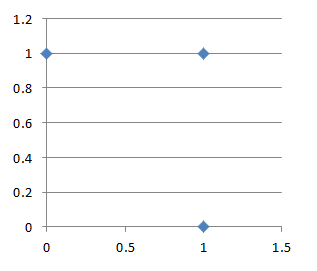
In a world of logical functions (we are building XOR classifier), this limitation means that a single layer perceptron is able to learn AND or OR function but it won't be able to learn XOR function.

One can easily imagine a line that separates all OR positive results from the negatives once. On the other hand there is no streight line that separates the positive XOR results ([0,1] and [1,0]) from the negatives ([0,0] and [1,1])

Feed forward multilayer networks

Feed forward network can be thought as composition of perceptrons. Such network has one input layer, multiple hidden layers and one output layer. The feed forward network does not contain cycles, unlike the Hopfield network in the next examples (which is recurrent neural network).

Unlike single layer perceptron, multilayer feed forward network is capable of learning linerably non-separable data such as the results of XOR function.

XOR classifier

This is the first example. This network is called clasifier because it learns the XOR function. It can then "classify" the 2 values in the input into single value on the output.

Here is how the network looks like:

The NN diagram was drawn in latex, using the tkz-berge package. Look here if you want to know how.

The network starts with random weights and continously updates the weights so that the result in the output node corresponds to the XOR of input values. In order to update the weights Backpropagation (Backwards propagation of errors) technique is used.

The value of the output is compared to the real value (which is known). The error is determined as the differences between the output and the real value. Then the weights of the edges has to be updated to minimalize the error as shown later.

Implementation

Each layer can be represented as one dimensional array, the weights are stored using 2-dimensional array ([0,1] is the weight between nodes 0 and 1). Here is the function which calculates the sum of values incomming to a single node and passes the value to the activation function. The activation function here can be any function, as it is passed as parameter but here Sigmoid is used.

let pass (input:float[]) (weights:float[,]) activation =
let length = weights |> Array2D.length2
seq {
 for i in 0 .. length-1 do
 let sum = (Array.zip weights.[*,i] input) |> Array.sumBy (fun (v,w) -> v * w)
 yield activation sum
} |> Array.ofSeq

By applying the pass multiple times, the whole network can be composed as sequence of pass functions.

The training procedure

The following function is the main loop of the XOR network and we iterate over until we obtain good results and the network is adapted.

let train network rate input target =
 let n1 = completepass input network
 let delta = deltaOutput n1.output target
 let deltaHidden = passDelta n1.hidden delta n1.hiddenToOutput
 let updatedHiddenToOut = updateWeights n1.hidden delta n1.hiddenToOutput rate
 let updatedInToHidden = updateWeights n1.input deltaHidden n1.inputToHidden rate

Completepass just calls 2 times the pass function value and gets the input values trough the hidden layer to the output. The output is then compared to desired result and error is estimated. From this error an array of "delta" values per each output node is determined which is then used to update the weights.

In the case of XOR network, there is only one output, so the delta will one dimensional array.

The delta has to be propagated lower so that we can also update the weights between the input and hidden layer.

Backpropagating the error

First the error of each layer has to be calculated. In the example bellow the error of the output layer is the value (t-o) or (Target - Ouput). This value is multiplied by value o*(1-o) which is the derivation of the Sigmoid function. The resulting array contains for each node a delta value, which shall be used to adjust the weights.

let deltaOutput (output:array<float>) (target:array<float>) =
 (Array.zip output target) |> Array.map (fun (o,t) -> o * (1.0 - o) * (t - o))

Delta propagation

Calculating the delta value for the output layer is not sufficient to correct all the weights in the network, the delta has to be propagated to the lower layers of the network, so that we can update the weights on the input - hidden connections.

let passDelta (outputs:float[]) (delta:float[]) (weights:float[,]) =
 let length = weights |> Array2D.length1
 seq {
 for i in 0 .. length-1 do
 let error = (Array.zip weights.[i,*] delta) |> Array.sumBy (fun (v,w) -> v * w)
 yield outputs.[i] * (1.0 - outputs.[i]) * error
 } |> Array.ofSeq

The "error" of the hidden layer is just the delta multiplied by the weight associated to the edge that propagates this delta to the lower value.

The last missing piece is the function that woudl update weights between 2 layers.

let updateWeights (layer:float[]) (delta:float[]) (weights:float[,]) learningRate =
 weights |> Array2D.mapi (fun i j w -> w + learningRate * delta.[j] * layer.[i])

Learning rate is a constant that determines how quickly the edges are updated. If the learning rate is too big, the network might miss the optimal weights. However if it is too small it will take longer time to get to the correct solution.

At the beginning the weight are set to random values between 0 and 1, or slided slightly. From the quick tests that I did it seems that for instance using learning rate of 0.3 it took 20000 iterations to get to a neural network that would XOR the values on it's inputs.

Hopfield-Tank network and Travelling Salesman Problem

TSP is one of the well known Combinatorial optimization problems and as such, it has been solved in many different ways (Integer Linear Programming, Genetic or Biologically inspired algorithms and other heuristics). Neural Networks are one of the many approaches to provide a solution to this problem.

Even within Neural Networks several different approaches have been developed to solve TSP (eg. elastic nets,self-organizing map). The approach demonstrated here is the oldest one: Hopfield neural network.

Hopfield neural network

Hopfield NN is a recurrent neural network (connections in the network form cycles). The units (nodes) in a Hopfield network can have only 2 values: 0|1 or -1|1 depending on literature, but in either case values that encode a binary state. The network is fully connected (each node is connected with any other node). The connection matrix is symetric, that is the weights on the edges are the same in both directions.

The initial Hopfied network had only binary values (0/1) but to solve TSP and for other problems continous version of the network is used, where every node has value in range [0,1].

The value of each node depends on the input potential of the node (Ui) and in order to keep it between (0,1) the tanh function is used:

The value of the input potential of each node depends on the values of all nodes that are connected to it and the values of the connections weights. This is actually identical to the way that the nodes in the XOR classifier behaved.

Network energy

Each state of the HNN can be described by a single value called Energy. While iterating and changing the state, the energy of HNN will either stay the same or will get smaller. The energy of the network will evenutelly convert to a local minimum - the state of the HNN that we target to solve the TSP

Hopfiled approach to TSP

The first and original approach to solve TSP was described in 1985 by Tank and Hopfield in their paper "Neural Computation of Decisions in Optimization Problems". Since then many more attempts were made. I have found these few papers or surweys available online quite useful and have used them to deduce my implementation:

• Jean-Yves Potvin - The Traveling Salesman Problem: A Neural Network Perspective
• Perspective of a neural optical solution of the Traveling Salesman optimization Problem
• Jacek Mandziuk -Solving the Travelling Salesman Problem with a Hopfield - type neural network

If I should pick one, I would say that the first one gave me most information about the problem, event though not enough implementation details. The others once then made it (almost) clear how to implement the solution.

Encoding TSP in Hopfield network

The neural network used to encode the TSP and it's solution is square matrix of nodes having N rows (one for each city) and N columns (one for each position in the tour), where N is the number of cities. When the algorithm finishes and the network converges to it's final state, each node will have value of either 0 or 1. As said the network in fully inter-connected so there is an edges between each node, which is not shown in the image bellow.

If the node in i-th row and j-th column has value 1, the city (i) will be in the tour on position (j).

As described above the network evolves and each node changes it's value over time. The secret of the algorithm is thus to provide such update rule that at the end the matrix of nodes will follow these criteria:

• Only one node in each row will have value 1
• Only one node in each column will have value 1
• There will be exactly N nodes having value 1
• The distances of the tour will be minimal

To come up with such update rule, Energy function has to be determine which will attain it's minimum for optimal solution of TSP. The energy function has to take into account the above specified rules. The following definition will satisfy the rules. Note that the following equations were taken from the J.Y Potvin's - paper

A,B,C and D are constants and the 4 sumations here correspond to the 4 above mentioned points.

Describing the dynamic of the network

There are two ways to describe the behaviour and the dynamic of the network:

• From the TSP energy function and the standard Hopfield network energy function we determine the weights between the nodes. Then we can let the network evolve over time. Since we have the weights of the connections between the nodes, we could iterate over the nodes, sum all the weighted inputs and set the output of the node. That would be an approach similar to the one taken on the XOR. This has one disadvantage, that is that the connection weights have to be determined from the equality between the standard Hopfield model enery function and the TSP Hopfield model function. There is an easier way without determining the connections weights.
• The easier way is to describe the change of the input potential without determining the weights of the edges. Then we can just iterate or randomly choose nodes, determine the new value of the potential and update the values of the connected nodes. This seems maybe ackward, because the network will evolve without having specific weighed connections between nodes. This options is described further.

The change in the node's input potential

One of the definition of the input potential of a node (i) can be described by:

What we want to determine, is how this value will change over time, when the network evolves. The change of the potential over time is it's partial derivation with respect to the time.

When doing a computer simulation we will described the value of Ui in time T+1, or here T+ delta t. Where delta T is some small time interval.

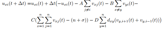
This equation is at the hearth of this algorithm. We now have an exact specification of what the value of potential Ui will be in time T+1. That is our iterating algorithm has to perfrom exactly this updated.

Implementation details

• Compute the distance matrix, containing the distance between each 2 cities
• Initialize the network with random values
• Pick randomly a node, compute the change in the input potential
• Update the value of the node from the input potential change
• Every n-iterations calculate the energy of the network
• Once the energy of the network stabilizes or you have reached fixed number of iterations - stop the process
• Translate the network into a city path

The network can be stored in 2-dimensional matrix. One can choose between storing the input potential of each node or the value of the each node, because the value of the node can be calculated from the potential at any time. I have chosen the second option and I store the input potential two dimensional array u.

The following code is the calculation of the input potential change of single node at coordinates (city,position). This is just retranscription of the equation above.

let singlePass (distances:float[,]) (u:float[,]) pms city position = 
 let n = Array2D.length2 u
 
 let values = u |> toValues pms
 let aSum = sumAllBut position (values |> rowi city)
 let bSum = sumAllBut city (values |> coli position)
 
 let cSum = (values |> Seq.cast<float> |> Seq.sum) - float(n+1)
 let dSum = dSumCalc distances city position values
 let dudt = -pms.A*aSum - pms.B*bSum - pms.C*cSum - pms.D*dSum
 //value of input potential in t+ delta_t
 let r = u.[city,position] + pms.dTime*(-u.[city,position] + dudt)
 //Alternatively according to the paper by Jacek Mandziuk one can just use the update value
 //let r = dudt
 r

There are few things to note. This code takes the distances matrix, the current state of the network (the value of input potential of each node), parameters of the network (constants A,B,C,D from equations above) and row (city) and the column (position) of the node that we are updating. The toValues method takes the current value of each node potential and returns a matrix of node values. The rowi and coli method return respecively one row or one column from 2 dimensional array. The sumAllBut method adds all elements of one-dimensional array except an element at position which is passed to the method. The dSumCalc method is the only one with a bit more compexity and it calculates the D value of the equation above (the one that assures the minimalization of the TSP circuit)

let rowi row (network:float[,]) = 
 network.[row,*] |> Array.mapi (fun j e -> (e,j))
let coli col (network:float[,]) = 
 network.[*,col] |> Array.mapi (fun j e -> (e,j))
let sumAllBut (i:int) (values:(float*int)[]) = 
 Array.fold (fun acc (e,j) -> if i<>j then acc + e else acc) 0.0 values
let dSumCalc distances city position (v:float[,]) = 
 let n = v |> Array2D.length1
 (distances |> rowi city) |> Array.sumBy (fun (e,i) -> 
 let index1 = (n+position+1) % n
 let index2 = (n+position-1) % n
 e*(v.[i,index1] + v.[i,index2])
 )
let toValues (pms:HopfieldTspParams) u = 
 u|> Array2D.map (fun (ui) -> v ui pms)
//calculates the value of node from input potential
let v (ui:float) (parameters:HopfieldTspParams) = (1.0 + tanh(ui*parameters.alfa))/2.0

The method which updates the input potential of single node can be called in 2 different ways. Either we pick the nodes randomly multiple times or we loop over all the nodes serially. If the update is serial then the only random element of the algorithm is the initialization of the netwok.

let serialIteration u pms distances = 
 u |> Array2D.mapi (fun i j x -> singlePass distances u pms i j)
let randomIteration u pms distances = 
 let r = new Random(DateTime.Now.Millisecond)
 let n = Array2D.length1 u
 for i in 0 .. 1000*n do
 let city = r.Next(n)
 let position = r.Next(n)
 u.[city, position] <- singlePass distances u pms city position
 u

The random iteration here is repeated 1000*n times where n is the number of cities, which is probably more than enough since the network seems to converge much sooner. Just for the sake of completeness, here is the method that runs 10 times either serial or random iteration.

let initAndRunUntilStable cities pms distances = 
 let u = initialize cities pms
 {1 .. 10} |> Seq.fold (fun uNext i -> 
 match pms.Update with
 | Random -> randomIteration uNext pms distances
 | Serial -> serialIteration uNext pms distances
 ) u

And here high level method, that generates a random example of TSP problem, calculates distances between all cities and runs the algorithm until a stable and correct solution is found. That is until the network returns feasable solution.

let sampleRun (pms:HopfieldTspParams ) (n:int) =
 let cities = generateRandomCities n
 let distances = calculateDistances cities
 let networks = Seq.initInfinite (fun i -> initAndRunUntilStable cities pms distances)
 let paths = networks |> Seq.map (fun v-> currentPath v)
 let validPath = paths |> Seq.find (fun path -> isFeasable path)
 cities, validPath

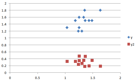
Results

The results are not overwhelming, on the other hand I have only implemented the most simple version of the algorithm. In the original paper the authors stated that the convergence rate to feasable solutions was about 50%. But depending on the parameters one can get better results. See bellow one of the runs of the algorithm on 6 random nodes.

Here is the complete list of parameters for Hopfield network and the values that I ended up using:

• Alpha: the parameters which shapes the Sigmoid decision function applied on each node (500)
• A: input potential change function, sum of rows (500)
• B: input potential change function, sum of columns (500)
• C: input potential change function, max N cities (200)
• D: input potential change function, minimalization of tour length (300)
• dTime: represents the delta T, the small update in time for each update of the input potential value (0.00001)

I have also used the standard update rule to obtain new value of the input potential which takes into account the current input potential.

 let dudt = -pms.A*aSum - pms.B*bSum - pms.C*cSum - pms.D*dSum
 //value of input potential in t+ delta_t
 u.[city,position] = u.[city,position] + pms.dTime*(-u.[city,position] + dudt)

According to the paper by Jacek Mandziuk one can just use the updated values as the new input potential, so that the update rule would become only:

 let dudt = -pms.A*aSum - pms.B*bSum - pms.C*cSum - pms.D*dSum
 u.[city,position] = dudt;

This rule didn't work for me. The convergance rate wasn't better neither were the tours lengths. Of course for such version, different values for network parameters have to be used.

Note that GitHub repostity and specifialy the Hopfield module contais more code:

• Method to determine the correct parameters. The performance of the algorithm greatly depends on the parameters of the Energy function and on the parameter alfa, which amplyfies the effect of the input potential on the value of given node.
• Few lines are also available to draw the solution using Windows Forms Charts, through F#

In a set of data points, outliers are such values that theoretically should not appear in the dataset. Typically these can be measurement errors or values caused by human mistakes. In some cases outliers are not caused by errors. These values affect the way that the data is treated and any statistics or report based on data containing outliers are erroneaus.

Detecting these values might be very hard or even impossible and a whole field of statistics called Robust Statistics covers this subject. If you are further interested into the subject please read Quantitative Data Cleaning For Large Databases written by Joseph M. Hellerstein from UC Barkeley. Everything that I have implemented here is taken from this paper. The only thing that I have added to that are two aggregates for SQL Server which help efficiently get the outliers and extreme values from the data stored in SQL Server and a simple tool to chart data and distribution of data using JavaScript

Theory

Any dataset can be characterized by the way the data is distributed over the whole range. The probability that a single point has given value in the dataset is defined using the probability distribution function. The Gaussian standard distribution is only one among many distribution functions, I won't go into statistics basics here, but let's consider only the standard distribution for our case.

In the Gaussian distribution the data points are somehow gathered around the "center", and most values fall not far. Rare are the values really far away from the center. Intuitively the ouliers are points very far from the center. Consider the following set of numbers which represent in minutes the length of a popular song:

3.9,3.8,3.9,2.7,2.8,1.9,2.7,3.5, 4.4, 2.8, 3.4, 8.6, 4.5, 3.5, 3.6, 3.8, 4.3, 4.5, 3.5,30,33,31

You have probably spotted the values 30,33 and 31 and you immediately identify them as outliers. Even if the Doors would double the length of their keyboard solo we would not get this far.

The standard distribution can be described using the probability density function. This function defines the probability that the point will have given value. The function is defined with two parameters: the center and the dispersion. The center is the most common value, the one around which all others are gathered. The dispersion describes how far the values are scattered from the center.

The probability that a point has a given value, provided that the data has the Gaussian distribution is given by this equation:

We can visualize both the theoretical and the real distribution of data. The distribution probability density function is continuous and thus can be charted as simple line. The distribution of the real data in turn can be visualized like a histogram.

The following graphics were created using KoExtensions project, which is a small mediator project making Knockout and D3 work nicely together.

In perfect world the center is the mean value. That value is probably not a part of a data set but represents the typical value. The seconds measure which describes how far from the center the data is dispersed is called standard deviation. If we want to obtain the standard deviation from data we take the distance of each point from the center, square these values add them together and take square root. So we actually have all we need to get the distribution parameters from the data.

This approach of course has one main flaw. The mean value is affected by the outliers. And since the dispersion is deduced using the mean and outliers affect the mean value, the dispersion as well will be affected by them. In order to get a description of the dataset not affected by the extreme values one needs to find robust replacements for the mean and the dispersion.

Robust Center

The simplest and very efficient replacement for the mean as the center of the data is the median. Median is such value that half of the points in the dataset are smaller are bellow. That is if the data set consists of even number of samples, we just need to order the values and take mean of the two values in the middle of the ordered array. If the data consist of odd number of values then we take the element exactly in the middle of the ordered data. The before mentioned paper describes two more alternatives: trimmed mean, winsorized mean. Both of these are based on the exclusion of marginal values and I did not used them in my implementation.

Let's take the median of the given dataset and see if the distribution function based on it fits better the data. Even though the center is now in correct place the shape of the function does not fit completely the data from the histogram. That is because the variance is still affected by the outliers.

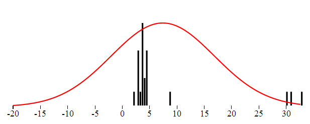
Robust Dispertion

Standard variance takes into account the the distance of all the numbers from the center. To rule out the extreme values, we can just use the median of distances. The outlier's distance from the center is much bigger than other distance and by taking the median of all distances we can get rid of outlier's influence over the dispersion. Here is the distribution function using this Robust type of dispersion. This characteristic is called MAD - Median Absolute Deviation.

Detecting the outliers

Now that we have the value of "real" center and "real spread" or dispersion we can state that the outlier is a value which differs "too much" from the center, taking into account the dispersion. Typically we could say that the outliers are such values that have a distance from center greater or equal to 10 * dispersion. The question is how to specify the multiplication coefficient. There is a statistics method called Hampel Indetifier which gives a formula to obtain the coefficient. Hampel identifier labels as outliers any points that are more than 5.2 away from the MAD. More details can be found here.

The overall reliability of this method

A question which might arise is up to which kind of messy data this method can be used. A common intuition would say that definitely more than the half of the data has to be "correct", in order to be able to detect the incorrect ones. To be able to measure the robustness of each method of detecting outliers, statisticians have introduced a term called Breakdown point. This point states which percentage of the data can be corrupted in order for given method to work. Using the Median as the center with the MAD (Median Absolute Deviation) has a breakdown point of 1/2. That is this method works if more than half of the data is correct. The standard arithmetic mean has a BP = 0. It is directly affected by all the numbers and one single outlier can completely move the data.

SQL implementation

In order to implement detection of outliers in SQL, one needs to first have the necessary functions to compute the mean, median and dispersion. All these functions are aggregates. Mean (avg) and Dispersion (var) are already implemented in SQL Server. If you are lucky enough to use SQL Server 2012 you can use the built-in median aggregate as well. The robust dispersion however has to be implemented manually even on SQL Server 2012.

Implementing aggregates for SQL Server is very easy, thanks to the predefined Visual Studio template. This templates will create a class for you which implements the IBinarySerializable interface and is decorate with couple attributes defined in the Microsoft.SqlServer namespace.

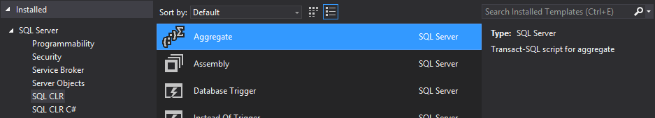
This class has 4 important methods:

• Init - anything needed before starting the aggregation
• Accumulate - adding one single value to the aggregate
• Merge - merging two aggregates
• Terminate - work to be done before returning the result of the aggregate

Here is the example of the Median aggregate

private List ld;
public void Init()
{
 ld = new List();
}
public void Accumulate(SqlDouble value)
{
 if (!value.IsNull)
 {
 ld.Add(value.Value);
 }
}
public void Merge(Median group)
{
 ld.AddRange(group.ld.ToArray());
}
public SqlDouble Terminate()
{
 return Tools.Median(ld);
}

Note that some aggregates can be computed iteratively. In that case all the necessary logic is in the Accumulate method and the Terminate method can be empty. With Median this is not the case (even though some iterative estimation methods exist. For the sake of the completeness, here is the implementation of median that I am using. It is the standard way: sorting the array and taking the middle element or average of the two middle elements. I am returning directly SqlDouble value, which is the result of the aggregate.

public static SqlDouble Median(List ld)
{
 if (ld.Count == 0)
 return SqlDouble.Null;
 ld.Sort();
 int index = ld.Count / 2;
 if (ld.Count % 2 == 0)
 {
 return (ld[index] + ld[index - 1]) / 2;
 }
 return ld[index];
}

Implementing the Robust variance using the MAD method is very similar, everything happens inside the Terminate method.

public SqlDouble Terminate()
{
 var distances = new List();
 var median = Tools.Median(ld);
 foreach (var item in ld)
 {
 var distance = Math.Abs(item - median.Value);
 distances.Add(distance);
 }
 var distMedian = Tools.Median(distances);
 return distMedian;
}

That implementation is directly the one described above: we take the distance of each element from the center (median) and than we take the median of the distances.

Outliers detection with the SQL aggregates

Having implemented both aggregates, detecting the outlier is just a matter of a SQL query - giving all the elements which are further away from the center than the variance multiplied by a coefficient.

select * from tbUsers where Height> ( Median(Height) + c*RobustVar(Height)) or Height < (Median(Height) - c*RobustVar(Height)) 

You will have to play with the coefficient value c to determine which multiplication gives you the best results.

JavaScript implementation

The same can be implemented in JavaScript. If you are interested in a JavaScript implementation you can check out the histogram chart from KoExtensions. This charting tool draws the histogram and the data distribution function. You can than configure it to use either Median or Mean as the center of the data as well as to use MAD, or standard variance to describe the dispersion.

KoExtensions is based on Knockout.JS and adds several useful bindings and the majority of them to simplify charting. Behind the scenes the data is charted using D3.

To draw a histogram chart with the distribution and detecting the outliers at the same time one needs just few lines of code

<div id="histogram" data-bind="histogram: data, chartOptions : {
 tolerance : 10,
 showProbabilityDistribution: true,min : -20,
 expected: 'median',
 useMAD: true,
 showOutliers: true}">

var exData = [3.9,3.8,3.9,2.7,2.8,1.9,2.7,3.5, 4.4, 2.8, 3.4, 8.6, 4.5, 3.5, 3.6, 3.8, 4.3, 4.5, 3.5,30,33,31];
 
function TestViewModel() {
 var self = this;
 self.data = ko.observableArray(exData);
}
var vm = new TestViewModel();
ko.applyBindings(vm);
initializeCharts();

Knockout.JS is a JavaScript MVVM framework tool which gives you all you need to create bi-directional binding between the view and the view model, where you can encapsulate and unit test all your logic. KoExtensions adds a binding call "histogram", which takes simple array and draws a histogram. In order to show the probability function and the outliers one has to set the options of the chart as shown in the example above.