Solving the NYTimes Pips puzzle with a constraint solver
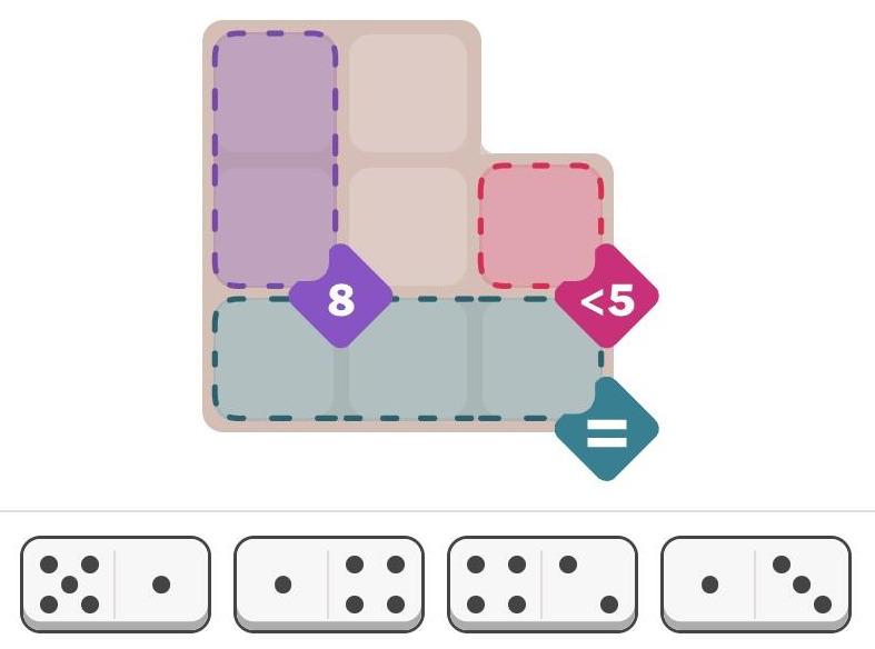
The New York Times recently introduced a new daily puzzle called Pips. You place a set of dominoes on a grid, satisfying various conditions. For instance, in the puzzle below, the pips (dots) in the purple squares must sum to 8, there must be fewer than 5 pips in the red square, and the pips in the three green squares must be equal. (It doesn't take much thought to solve this "easy" puzzle, but the "medium" and "hard" puzzles are more challenging.)
I was wondering about how to solve these puzzles with a computer. Recently, I saw an article on Hacker News—"Many hard LeetCode problems are easy constraint problems"—that described the benefits and flexibility of a system called a constraint solver. A constraint solver takes a set of constraints and finds solutions that satisfy the constraints: exactly what Pips requires.
I figured that solving Pips with a constraint solver would be a good way to learn more about these solvers, but I had several questions. Did constraint solvers require incomprehensible mathematics? How hard was it to express a problem? Would the solver quickly solve the problem, or would it get caught in an exponential search?
It turns out that using a constraint solver was straightforward; it took me under two hours from knowing nothing about constraint solvers to solving the problem. The solver found solutions in milliseconds (for the most part). However, there were a few bumps along the way. In this blog post, I'll discuss my experience with the MiniZinc 1 constraint modeling system and show how it can solve Pips.
Approaching the problem
Writing a program for a constraint solver is very different from writing a regular program. Instead of telling the computer how to solve the problem, you tell it what you want: the conditions that must be satisfied. The solver then "magically" finds solutions that satisfy the problem.
To solve the problem, I created an array called pips that holds the number of domino pips at each position
in the grid.
Then, the three constraints for the above problem can be expressed as follows.
You can see how the constraints directly express the conditions in the puzzle.
constraint pips[1,1] + pips[2,1] == 8;
constraint pips[2,3] < 5; constraint all_equal([pips[3,1], pips[3,2], pips[3,3]]);
Next, I needed to specify where dominoes could be placed for the puzzle.
To do this, I defined an array called grid that indicated the allowable positions: 1 indicates a valid
position and 0 indicates an invalid position. (If you compare with the puzzle at the top of the article,
you can see that the grid below matches its shape.)
grid = [|
1,1,0|
1,1,1|
1,1,1|];
I also defined the set of dominoes for the problem above, specifying the number of spots in each half:
spots = [|5,1| 1,4| 4,2| 1,3|];
So far, the constraints directly match the problem.
However, I needed to write some more code to specify how these pieces interact.
But
before I describe that code, I'll show a solution.
I wasn't sure what to expect: would the constraint solver give me a solution or would it spin
forever?
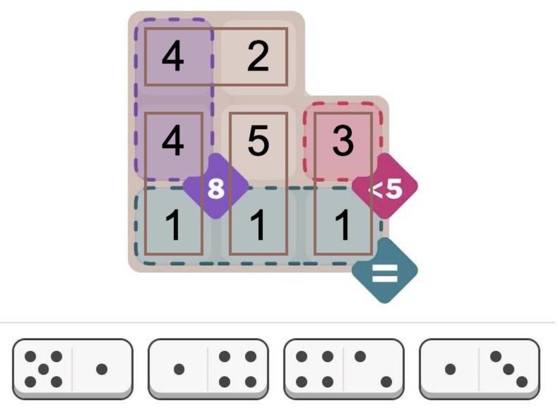
It turned out to find the unique solution in 109 milliseconds, printing out the
solution arrays.
The pips array shows the number of pips in each position, while the dominogrid array shows which
domino (1 through 4) is in each position.
pips =
[| 4, 2, 0
 | 4, 5, 3
 | 1, 1, 1
 |];
dominogrid =
[| 3, 3, 0
 | 2, 1, 4
 | 2, 1, 4
 |];
The text-based solution above is a bit ugly. But it is easy to create graphical output. MiniZinc provides a JavaScript API, so you can easily display solutions on a web page. I wrote a few lines of JavaScript to draw the solution, as shown below. (I just display the numbers since I was too lazy to draw the dots.) Solving this puzzle is not too impressive—it's an "easy" puzzle after all—but I'll show below that the solver can also handle considerably more difficult puzzles.
Graphical display of the solution.
Details of the code
While the above code specifies a particular puzzle, a bit more code is required to define how dominoes and the grid interact. This code may appear strange because it is implemented as constraints, rather than the procedural operations in a normal program.
My main design decision was how to specify the locations of dominoes.
I considered assigning a grid position and orientation
to each domino, but it seemed inconvenient to deal with multiple orientations.
Instead, I decided to position each half of the domino independently, with an x and y coordinate in
the grid.2 I added a constraint that the two halves of each domino had to be in neighboring cells,
that is, either the X or Y coordinates had to differ by 1.
constraint forall(i in DOMINO) (abs(x[i, 1] - x[i, 2]) + abs(y[i, 1] - y[i, 2]) == 1);
It took a bit of thought to fill in the pips array with the number of spots on each domino.
In a normal programming language, one would loop over the dominoes and store the values into pips.
However, here it is done with a constraint so the solver makes sure the values are assigned.
Specifically, for each half-domino, the pips array entry at
the domino's x/y coordinate must equal the corresponding spots on the domino:
constraint forall(i in DOMINO, j in HALF) (pips[y[i,j], x[i, j]] == spots[i, j]);
I decided to add another array to keep track of which domino is in which position.
This array is useful to see the domino locations in the output, but it also
keeps dominoes from overlapping.
I used a constraint to put each domino's number (1, 2, 3, etc.) into the occupied position of dominogrid:
constraint forall(i in DOMINO, j in HALF) (dominogrid[y[i,j], x[i, j]] == i);
Next, how do we make sure that dominoes only go into positions allowed by grid?
I used a constraint that a square in dominogrid must be empty or the corresponding grid must allow a domino.3
This uses the "or" condition, which is expressed as \/, an unusual stylistic
choice. (Likewise, "and" is expressed as /\. These correspond to the logical symbols
∨ and ∧.)
constraint forall(i in 1..H, j in 1..W) (dominogrid[i, j] == 0 \/ grid[i, j] != 0);
Honestly, I was worried that I had too many arrays and the solver would end up in a rathole ensuring that the arrays were consistent. But I figured I'd try this brute-force approach and see if it worked. It turns out that it worked for the most part, so I didn't need to do anything more clever.
Finally, the program requires a few lines to define some constants and variables. The constants below define the number of dominoes and the size of the grid for a particular problem:
int: NDOMINO = 4; % Number of dominoes in the puzzle
int: W = 3; % Width of the grid in this puzzle
int: H = 3; % Height of the grid in this puzzle
Next, datatypes are defined to specify the allowable values.
This is very important for the solver; it is a "finite domain" solver, so limiting the size of
the domains reduces the size of the problem.
For this problem, the values are integers in a particular range, called a set:
set of int: DOMINO = 1..NDOMINO; % Dominoes are numbered 1 to NDOMINO
set of int: HALF = 1..2; % The domino half is 1 or 2
set of int: xcoord = 1..W; % Coordinate into the grid
set of int: ycoord = 1..H;
At last, I define the sizes and types of the various arrays that I use.
One very important syntax is var, which indicates variables that the solver must determine.
Note that the first two arrays, grid and spots do not have var since they are constant,
initialized to specify the problem.
array[1..H,1..W] of 0..1: grid; % The grid defining where dominoes can go
array[DOMINO, HALF] of int: spots; % The number of spots on each half of each domino
array[DOMINO, HALF] of var xcoord: x; % X coordinate of each domino half
array[DOMINO, HALF] of var ycoord: y; % Y coordinate of each domino half
array[1..H,1..W] of var 0..6: pips; % The number of pips (0 to 6) at each location.
array[1..H,1..W] of var 0..NDOMINO: dominogrid; % The domino sequence number at each location
You can find all the code on GitHub.
One weird thing is that because the code is not procedural, the lines can be in any order.
You can use arrays or constants before you use them.
You can even move include statements to the end of the file if you want!
Complications
Overall, the solver was much easier to use than I expected. However, there were a few complications.
By changing a setting, the solver can find multiple solutions instead of stopping after the first. However, when I tried this, the solver generated thousands of meaningless solutions. A closer look showed that the problem was that the solver was putting arbitrary numbers into the "empty" cells, creating valid but pointlessly different solutions. It turns out that I didn't explicitly forbid this, so the sneaky constraint solver went ahead and generated tons of solutions that I didn't want. Adding another constraint fixed the problem. The moral is that even if you think your constraints are clear, solvers are very good at finding unwanted solutions that technically satisfy the constraints. 4
A second problem is that if you do something wrong, the solver simply says that the problem is unsatisfiable. Maybe there's a clever way of debugging, but I ended up removing constraints until the problem can be satisfied, and then see what I did wrong with that constraint. (For instance, I got the array indices backward at one point, making the problem insoluble.)
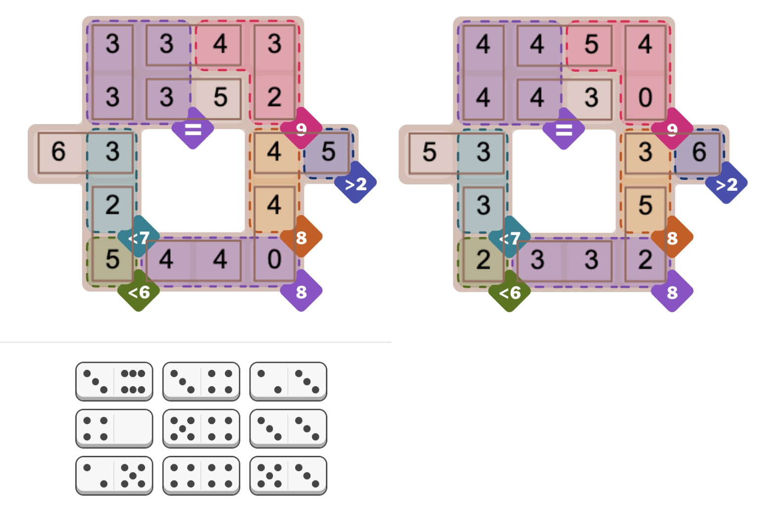
The most concerning issue is the unpredictability of the solver: maybe it will take milliseconds or maybe it will take hours. For instance, the Oct 5 hard Pips puzzle (below) caused the solver to take minutes for no apparent reason. However, the MiniZinc IDE supports different solver backends. I switched from the default Gecode solver to Chuffed, and it immediately found numerous solutions, 384 to be precise. (Sometimes the Pips puzzles sometimes have multiple solutions, which players find controversial.) I suspect that the multiple solutions messed up the Gecode solver somehow, perhaps because it couldn't narrow down a "good" branch in the search tree. For a benchmark of the different solvers, see the footnote.5
Two of the 384 solutions to the NYT Pips puzzle from Oct 5, 2025 (hard difficulty).
How does a constraint solver work?
If you were writing a program to solve Pips from scratch, you'd probably have a loop to try assigning dominoes to positions. The problem is that the problem grows exponentially. If you have 16 dominoes, there are 16 choices for the first domino, 15 choices for the second, and so forth, so about 16! combinations in total, and that's ignoring orientations. You can think of this as a search tree: at the first step, you have 16 branches. For the next step, each branch has 15 sub-branches. Each sub-branch has 14 sub-sub-branches, and so forth.
An easy optimization is to check the constraints after each domino is added. For instance, as soon as the "less than 5" constraint is violated, you can backtrack and skip that entire section of the tree. In this way, only a subset of the tree needs to be searched; the number of branches will be large, but hopefully manageable.
A constraint solver works similarly, but in a more abstract way. The constraint solver assigns values to the variables, backtracking when a conflict is detected. Since the underlying problem is typically NP-complete, the solver uses heuristics to attempt to improve performance. For instance, variables can be assigned in different orders. The solver attempts to generate conflicts as soon as possible so large pieces of the search tree can be pruned sooner rather than later. (In the domino case, this corresponds to placing dominoes in places with the tightest constraints, rather than scattering them around the puzzle in "easy" spots.)
Another technique is constraint propagation. The idea is that you can derive new constraints and catch conflicts earlier. For instance, suppose you have a problem with the constraints "a equals c" and "b equals c". If you assign "a=1" and "b=2", you won't find a conflict until later, when you try to find a value for "c". But with constraint propagation, you can derive a new constraint "a equals b", and the problem will turn up immediately. (Solvers handle more complicated constraint propagation, such as inequalities.) The tradeoff is that generating new constraints takes time and makes the problem larger, so constraint propagation can make the solver slower. Thus, heuristics are used to decide when to apply constraint propagation.
Researchers are actively developing new algorithms, heuristics, and optimizations6 such as backtracking more aggressively (called "backjumping"), keeping track of failing variable assignments (called "nogoods"), and leveraging Boolean SAT (satisfiability) solvers. Solvers compete in annual challenges to test these techniques against each other. The nice thing about a constraint solver is that you don't need to know anything about these techniques; they are applied automatically.
Conclusions
I hope this has convinced you that constraint solvers are interesting, not too scary, and can solve real problems with little effort. Even as a beginner, I was able to get started with MiniZinc quickly. (I read half the tutorial and then jumped into programming.)
One reason to look at constraint solvers is that they are a completely different programming paradigm. Using a constraint solver is like programming on a higher level, not worrying about how the problem gets solved or what algorithm gets used. Moreover, analyzing a problem in terms of constraints is a different way of thinking about algorithms. Some of the time it's frustrating when you can't use familiar constructs such as loops and assignments, but it expands your horizons.
Finally, writing code to solve Pips is more fun than solving the problems by hand, at least in my opinion, so give it a try!
For more, follow me on Bluesky (@righto.com), Mastodon (@[email protected]), RSS, or subscribe here.
all_equal and alldifferent constraint functions.Notes and references
-
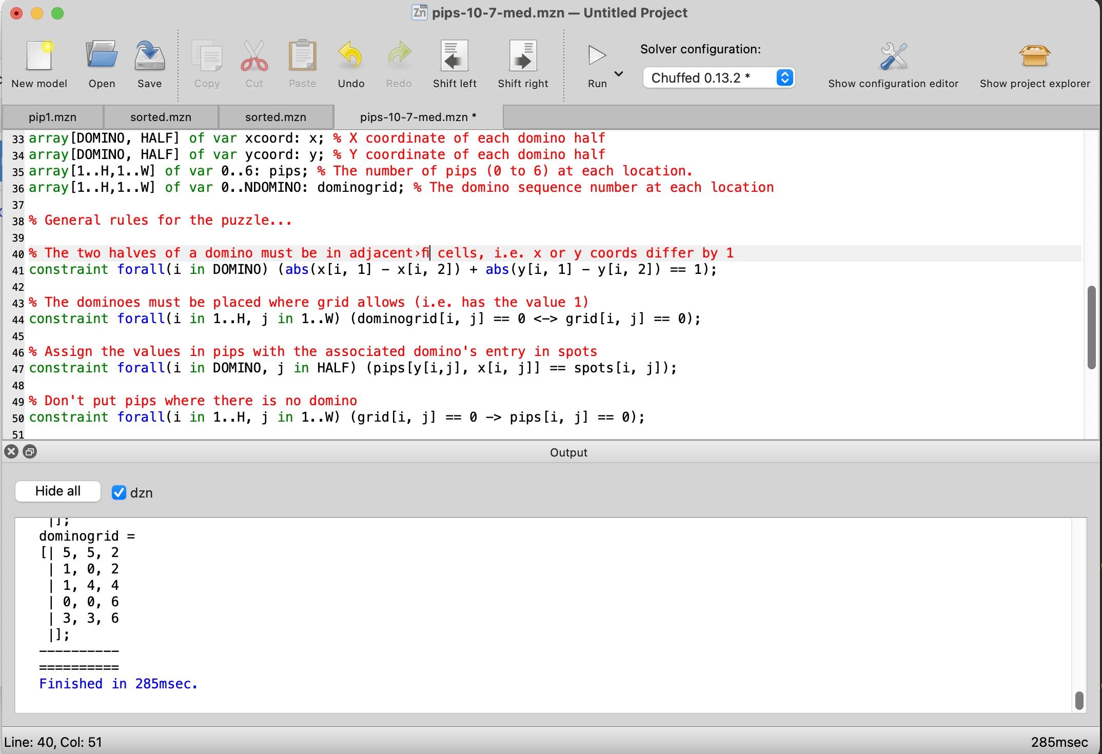
I started by downloading the MiniZinc IDE and reading the MiniZinc tutorial. The MiniZinc IDE is straightforward, with an editor window at the top and an output window at the bottom. Clicking the "Run" button causes it to generate a solution.
Screenshot of the MiniZinc IDE. Click for a larger view.
Screenshot of the MiniZinc IDE. Click for a larger view. -
It might be cleaner to combine the X and Y coordinates into a single
Pointtype, using a MiniZinc record type. ↩ -
I later decided that it made more sense to enforce that
dominogridis empty if and only ifgridis 0 at that point, although it doesn't affect the solution. This constraint uses the "if and only if" operator<->.constraint forall(i in 1..H, j in 1..W) (dominogrid[i, j] == 0 <-> grid[i, j] == 0);
↩ -
To prevent the solver from putting arbitrary numbers in the unused positions of
pips, I added a constraint to force these values to be zero:constraint forall(i in 1..H, j in 1..W) (grid[i, j] == 0 -> pips[i, j] == 0);
Generating multiple solutions had a second issue, which I expected: A symmetric domino can be placed in two redundant ways. For instance, a double-six domino can be flipped to produce a solution that is technically different but looks the same. I fixed this by adding constraints for each symmetric domino to allow only one of the two redundant positions. The constraint below forces a preferred orientation for symmetric dominoes.
constraint forall(i in DOMINO) (spots[i,1] != spots[i,2] \/ x[i,1] > x[i,2] \/ (x[i,1] == x[i,2] /\ y[i,1] > y[i,2]));
To enable multiple solutions in MiniZinc, the setting is under Show Configuration Editor > User Defined Behavior > Satisfaction Problems or the
--allflag from the command line. ↩ -
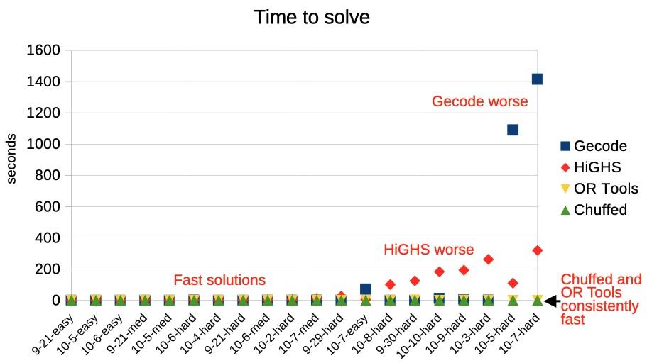
MiniZinc has five solvers that can solve this sort of integer problem: Chuffed, OR Tools CP-SAT, Gecode, HiGHS, and Coin-OR BC. I measured the performance of the five solvers against 20 different Pips puzzles. Most of the solvers found solutions in under a second, most of the time, but there is a lot of variation.
Timings for different solvers on 20 Pip puzzles.
Timings for different solvers on 20 Pip puzzles.Overall, Chuffed had the best performance on the puzzles that I tested, taking well under a second. Google's OR-Tools won all the categories in the 2025 MiniZinc challenge, but it was considerably slower than Chuffed for my Pips programs. The default Gecode solver performed very well most of the time, but it did terribly on a few problems, taking over 15 minutes. HiGHs was slower in general, taking a few minutes on the hardest problems, but it didn't fail as badly as Gecode. (Curiously, Gecode and HiGHS sometimes found different problems to be difficult.) Finally, Coin-OR BC was uniformly bad; at best it took a few seconds, but one puzzle took almost two hours and others weren't solved before I gave up after two hours. (I left Coin-OR BC off the graph because it messed up the scale.)
Don't treat these results too seriously because different solvers are optimized for different purposes. (In particular, Coin-OR BC is designed for linear problems.) But the results demonstrate the unpredictability of solvers: maybe you get a solution in a second and maybe you get a solution in hours. ↩
-
If you want to read more about solvers, Constraint Satisfaction Problems is an overview presentation. The Gecode algorithms are described in a nice technical report: Constraint Programming Algorithms used in Gecode. Chuffed is more complicated: "Chuffed is a state of the art lazy clause solver designed from the ground up with lazy clause generation in mind. Lazy clause generation is a hybrid approach to constraint solving that combines features of finite domain propagation and Boolean satisfiability." The Chuffed paper Lazy clause generation reengineered and slides are more of a challenge. ↩
Why do people keep writing about the imaginary compound Cr2Gr2Te6?
I was reading the latest issue of the journal Science, and a paper mentioned the compound Cr2Gr2Te6. For a moment, I thought my knowledge of the periodic table was slipping, since I couldn't remember the element Gr. It turns out that Gr was supposed to be Ge, germanium, but that raises two issues. First, shouldn't the peer reviewers and proofreaders at a top journal catch this error? But more curiously, it appears that this formula is a mistake that has been copied around several times.
The Science paper [1] states, "Intrinsic ferromagnetism in these materials was discovered in Cr2Gr2Te6 and CrI3 down to the bilayer and monolayer thickness limit in 2017." I checked the referenced paper [2] and verified that the correct compound is Cr2Ge2Te6, with Ge for germanium.
But in the process, I found more publications that specifically mention the 2017 discovery of intrinsic ferromagnetism in both Cr2Gr2Te6 and CrI3. A 2021 paper in Nanoscale [3] says, "Since the discovery of intrinsic ferromagnetism in atomically thin Cr2Gr2Te6 and CrI3 in 2017, research on two-dimensional (2D) magnetic materials has become a highlighted topic." Then, a 2023 book chaper [4] opens with the abstract: "Since the discovery of intrinsic long-range magnetic order in two-dimensional (2D) layered magnets, e.g., Cr2Gr2Te6 and CrI3 in 2017, [...]"
This illustrates how easy it is for a random phrase to get copied around with nobody checking it. (Earlier, I found a bogus computer definition that has persisted for over 50 years.) To be sure, these could all be independent typos—it's an easy typo to make since Ge and Gr are neighbors on the keyboard and Cr2Gr2 scans better than Cr2Ge2. A few other papers [5, 6, 7] have the same typo, but in different contexts. My bigger concern is that once AI picks up the erroneous formula, it will propagate as misinformation forever. I hope that by calling out this error, I can bring an end to it. In any case, if anyone ends up here after a web search, I can at least confirm that there isn't a new element Gr and the real compound is Cr2Ge2Te6, chromium germanium telluride.
References
[1] He, B. et al. (2025) ‘Strain-coupled, crystalline polymer-inorganic interfaces for efficient magnetoelectric sensing’, Science, 389(6760), pp 623-631. (link)
[2] Gong, C. et al. (2017) ‘Discovery of intrinsic ferromagnetism in two-dimensional van der Waals crystals’, Nature, 546(7657), pp. 265–269. (link)
[3] Zhang, S. et al. (2021) ‘Two-dimensional magnetic materials: structures, properties and external controls’, Nanoscale, 13(3), pp. 1398–1424. (link)
[4] Yin, T. (2024) ‘Novel Light-Matter Interactions in 2D Magnets’, in D. Ranjan Sahu (ed.) Modern Permanent Magnets - Fundamentals and Applications. (link)
[5] Zhao, B. et al. (2023) ‘Strong perpendicular anisotropic ferromagnet Fe3GeTe2/graphene van der Waals heterostructure’, Journal of Physics D: Applied Physics, 56(9) 094001. (link)
[6] Ren, H. and Lan, M. (2023) ‘Progress and Prospects in Metallic FexGeTe2 (3≤x≤7) Ferromagnets’, Molecules, 28(21), p. 7244. (link)
[7] Hu, S. et al. (2019) 'Anomalous Hall effect in Cr2Gr2Te6/Pt hybride structure', Taiwan-Japan Joint Workshop on Condensed Matter Physics for Young Researchers, Saga, Japan. (link)
Wealth distribution in the United States
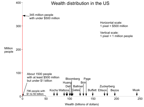
Forbes recently published the Forbes 400 List for 2024, listing the 400 richest people in the United States. This inspired me to make a histogram to show the distribution of wealth in the United States. It turns out that if you put Elon Musk on the graph, almost the entire US population is crammed into a vertical bar, one pixel wide. Each pixel is 500ドル million wide, illustrating that 500ドル million essentially rounds to zero from the perspective of the wealthiest Americans.
[画像:Graph showing the wealth distribution in the United States.]
The histogram above shows the wealth distribution in red. Note that the visible red line is one pixel wide at the left and disappears everywhere else—this is the important point: essentially the entire US population is in that first bar. The graph is drawn with the scale of 1 pixel = 500ドル million in the X axis, and 1 pixel = 1 million people in the Y axis. Away from the origin, the red line is invisible—a tiny fraction of a pixel tall since so few people have more than 500 million dollars.
Since the median US household wealth is about 190,000,ドル half the population would be crammed into a microscopic red line 1/2500 of a pixel wide using the scale above. (The line would be much narrower than the wavelength of light so it would be literally invisible). The very rich are so rich that you could take someone with a thousand times the median amount of money, and they would still have almost nothing compared to the richest Americans. If you increased their money by a factor of a thousand yet again, you'd be at Bezos' level, but still well short of Elon Musk.
Another way to visualize the extreme distribution of wealth in the US is to imagine everyone in the US standing up while someone counts off millions of dollars, once per second. When your net worth is reached, you sit down. At the first count of 1ドル million, most people sit down, with 22 million people left standing. As the count continues—2ドル million, 3ドル million, 4ドル million—more people sit down. After 6 seconds, everyone except the "1%" has taken their seat. As the counting approaches the 17-minute mark, only billionaires are left standing, but there are still days of counting ahead. Bill Gates sits down after a bit over one day, leaving 8 people, but the process is nowhere near the end. After about two days and 20 hours of counting, Elon Musk finally sits down.
Sources
The main source of data is the Forbes 400 List for 2024. Forbes claims there are 813 billionaires in the US here. Median wealth data is from the Federal Reserve; note that it is from 2022 and household rather than personal. The current US population estimate is from Worldometer. I estimated wealth above 500ドル million, extrapolating from 2019 data.
I made a similar graph in 2013; you can see my post here for comparison.
Disclaimers: Wealth data has a lot of sources of error including people vs households, what gets counted, and changing time periods, but I've tried to make this graph as accurate as possible. I'm not making any prescriptive judgements here, just presenting the data. Obviously, if you want to see the details of the curve, a logarithmic scale makes more sense, but I want to show the "true" shape of the curve. I should also mention that wealth and income are very different things; this post looks strictly at wealth.
Intel x86 documentation has more pages than the 6502 has transistors
It turns out that Intel's Intel® 64 and IA-32 Architectures Software Developer Manuals (2011) have 4181 pages in total, while the 6502 has 3510 transistors. There are actually more pages of documentation for the x86 than the number of individual transistors in the 6502.
The above photo shows Intel's IA-32 software developer's manuals from 2004 on top of the 6502 chip's schematic. Since then the manuals have expanded to 7 volumes.
The 6502 has 3510 transistors, or 4528, or 6630, or maybe 9000?
As a slight tangent, it's actually hard to define the transistor count of a chip. The 6502 is usually reported as having 3510 transistors. This comes from the Visual 6502 team, which dissolved a 6502 chip in acid, photographed the die (below), traced every transistor in the image, and built a transistor-level simulator that runs 6502 code (which you really should try). Their number is 3510 transistors.
One complication is the 6502 is built with NMOS logic which builds gates out of active "enhancement" transistors as well as pull-up "depletion" transistors which basically act as resistors. The count of 3510 is just the enhancement transistors. If you include the (削除) 2102 (削除ここまで) 1018 depletion transistors, the total transistor count is (削除) 5612 (削除ここまで) 4528.
A second complication is that when manufacturers report the transistor count of chips, they often report "potential" transistors. Chips that include a ROM or PLA will have different numbers of transistors depending on the values stored in the ROM. Since marketing doesn't want to publish different transistor numbers depending on the number of 1 bits and 0 bits programmed into the chip, they often count ROM or PLA sites: places that could have transistors, but might not. By my count, the 6502 decode PLA has 21×131=2751 PLA sites, of which 649 actually have transistors. Adding these 2102 "potential" transistors yields a count of 6630 transistors.
Finally, some sources such as Microsoft Encarta and A History of the Personal Computer state the 6502 contains 9000 transistors, but I don't know how they could have come up with that value.
(The number of pages of Intel documentation is also not constant; the latest 2013 Software Developer Manuals have shrunk to 3251 pages.)
Thus, the x86 has more pages of documentation than the 6502 has transistors, but it depends how you count.
9 Hacker News comments I'm tired of seeing
- Correlation is not causation: the few readers who don't know this already won't benefit from mentioning it. If there's some specific reason you think a a study is wrong, describe it.
- "If you're not paying for it, you're the product" - That was insightful the first time, but doesn't need to be posted about every free website.
- Explaining a company's actions by "the legal duty to maximize shareholder value" - Since this can be used to explain any action by a company, it explains nothing. Not to mention the validity of the statement is controversial.
- [citation needed] - This isn't Wikipedia, so skip the passive-aggressive comments. If you think something's wrong, explain why.
- Premature optimization - labeling every optimization with this vaguely Freudian phrase doesn't make you the next Knuth. Calling every abstraction a leaky abstraction isn't useful either.
- Dunning-Kruger effect - an overused explanation and criticism.
- Betteridge's law of headlines - this comment doesn't need to appear every time a title ends in a question mark.
- A link to a logical fallacy, such as ad hominem or more pretentiously tu quoque - this isn't a debate team and you don't score points for this.
- "Cue the ...", "FTFY", "This.", "+1", "Sigh", "Meh", and other generic internet comments are just annoying.
- The plural of anecdote is not data
- Cargo cult
- Comments starting with "No." "Wrong." or "False."
- Just use bootstrap / heroku / nodejs / Haskell / Arduino.
- "How [or Why] did this make the front page of HN?" followed by http://ycombinator.com/newsguidelines.html
What comments bother you the most?
Amusing note: when I saw the comments below, I almost started deleting them thinking "These are the stupidest comments I've seen in a long time". Then I realized I'd asked for them :-)
There are three basic types of online participants: "watercooler", "scientific conference", and "debate team". In "watercooler", the participants are having an entertaining conversation and sharing anecdotes. In "scientific conference", the participants are trying to increase knowledge and solve problems. In "debate team", the participants are trying to prove their point is right.
HN was originally largely in the "scientific conference" mode, with very smart people discussing areas in which they were experts. Now HN has much more "watercooler" flavor, with smart people chatting about random things they often know little about. And certain subjects (e.g. economics, Apple, sexism, piracy) bring out the "debate team" commenters. Any of the three types can carry on happily by themself. However, much of the problem comes when the types of conversation mix. The "watercooler" conversations will annoy the "scientific conference" readers, since half of what they say is wrong. Conversely, the "scientific conference" commenters come across as pedantic when they interrupt a fun conversation with facts and corrections. A conversation between "debate team" and one of the other groups obviously goes nowhere.
Wealth distribution in the United States
This graph shows the wealth distribution in red. Note that the visible red line is one pixel wide and disappears everywhere else - this is the key point: essentially the entire US population is in that first bar. The graph is drawn with the scale of 1 pixel = 100ドル million in the X axis, and 1 pixel = 1 million people in the Y axis. Away from the origin, the red line is invisible - less than 1/1000 of a pixel tall since so few people have more than 100ドル million dollars. It's striking just how much money Bill Gates has; even 100ドル million is negligible in comparison.
Since the median US household wealth is about 100,000,ドル half the population is crammed into a microscopic red line 1/1000 of a pixel wide. (The line would be narrower than the wavelength of light so it would be literally invisible). And it turns out the 1-pixel-wide red line isn't just the "99%", but the 99.999%. I hypothesize this is why even many millionaires don't feel rich.
Wealth inequality among billionaires
Much has been written about inequality in the US between the rich and the poor, but it turns out there is also huge inequality among the ranks of billionaires. Looking at the 1.9 trillion dollars held by US billionaires, it turns out that the top 20% of billionaires have 59% of this wealth, while the bottom 20% of billionaires have less than 6%. So even among billionaires, most of the money is skewed to the top. (I originally pointed this out in Forbes in 1998, and the billionaire inequality has grown slightly since then.)Sources
The billionaire data is from Forbes billionaires list 2013. Median wealth is from Wikipedia. Also Measuring the Top 1% by Wealth, Not Income and More millionaires despite tough times. Wealth data has a lot of sources of error including people vs households, what gets counted, and changing time periods, but I've tried to make this graph as accurate as possible. I should also mention that wealth and income are two very different things; this post looks strictly at wealth.The Mathematics of Volleyball
I decided to analyze the game mathematically. I made the simplifying assumption that each team had 50-50 odds of winning each point. I found the analysis interesting, and it turns out to have close ties to Pascal's Triangle, so I'm posting it here in case anyone else is interested.
Volleyball games are scored using the rally point system, which means that one team gets a point on every serve. (Back in the olden days, volleyball used side-out scoring, which meant that only the serving team could get a point. Fortunately, rally point scoring is more mathematically tractable. Rally point scoring also keeps the game advancing faster.) The winner of each match is the best out of three sets (a set is the same as a game). In the league I was watching, the winner of a game is the first team to get 25 points and be ahead by at least 2. (Except if a third tiebreaker game is needed, it only goes to 15 points instead of 25.)
A few cases are easy to analyze mathematically. If we assume each team has a 50-50 chance of scoring each point and the score is tied, each team obviously has a 50% chance of winning the game. (With side-out scoring, it makes a difference which team is serving, but for rally point scoring we avoid that complication.) The second obvious case is if a team has 25 points and the other team has 23 or fewer points, the first team has 100% chance of winning (since they already won).
I will use the notation P(m,n) for the chance of the first team wining if the score is m to n. From above, P(n, n) = 50%, P(25, n) = 100% for n <= 23, and P(m, 25) = 0% for m <= 23.
The chance of winning in other cases can be calculated from the assumption that a team has a 50% chance of winning the point, and a 50% chance of losing: the chance of winning is the average of these two circumstances. Mathematically, we get the simple recurrence:
For instance, if the score is 25-24, if the first team scores, they win. If the second team scores, then the score is tied. In the first (winning) case, the first team wins 100%, and in the second (tied) case, the first team wins 50%. Thus, on average they will win 75% of the time from a 25-24 lead. That is, P(25, 24) = 75%, and by symmetry P(24, 25) = 25%. (Surprisingly, these are the only scores where the requirement to win by 2 points changes the odds.)
Likewise, if the score is 24-23, half the time the first team will score a point and win, and half the time the second team will score a point and tie. So the first team has 1/2 * 100% + 1/2 * 50% = 75% chance of winning, and P(24, 23) = 75%.
More interesting is if the score is 24-22, half the time the first team will score a point and win, and half the time the second team will score, making the score 24-23. We know from above that the first team has a 75% chance of winning from 24-23, so P(24, 22) = 1/2 * 100% + 1/2 * 75% = 87.5%.
We can use the recurrence to work backwards and find the probability of winning from any score. The following table shows the probability of winning for each score. The first team has the score on the left, and the second team has the score on the top.
Table with odds of winning when the score is m to n
| 0 | 1 | 2 | 3 | 4 | 5 | 6 | 7 | 8 | 9 | 10 | 11 | 12 | 13 | 14 | 15 | 16 | 17 | 18 | 19 | 20 | 21 | 22 | 23 | 24 | 25 | |
|---|---|---|---|---|---|---|---|---|---|---|---|---|---|---|---|---|---|---|---|---|---|---|---|---|---|---|
| 0 | 50% | 44% | 39% | 33% | 28% | 23% | 18% | 14% | 11% | 8% | 5% | 4% | 2% | 1% | 1% | 0% | 0% | 0% | 0% | 0% | 0% | 0% | 0% | 0% | 0% | 0% |
| 1 | 56% | 50% | 44% | 38% | 33% | 27% | 22% | 17% | 13% | 10% | 7% | 5% | 3% | 2% | 1% | 1% | 0% | 0% | 0% | 0% | 0% | 0% | 0% | 0% | 0% | 0% |
| 2 | 61% | 56% | 50% | 44% | 38% | 32% | 27% | 21% | 17% | 13% | 9% | 7% | 4% | 3% | 2% | 1% | 1% | 0% | 0% | 0% | 0% | 0% | 0% | 0% | 0% | 0% |
| 3 | 67% | 62% | 56% | 50% | 44% | 38% | 32% | 26% | 21% | 16% | 12% | 9% | 6% | 4% | 3% | 1% | 1% | 0% | 0% | 0% | 0% | 0% | 0% | 0% | 0% | 0% |
| 4 | 72% | 67% | 62% | 56% | 50% | 44% | 37% | 31% | 26% | 20% | 16% | 11% | 8% | 6% | 4% | 2% | 1% | 1% | 0% | 0% | 0% | 0% | 0% | 0% | 0% | 0% |
| 5 | 77% | 73% | 68% | 62% | 56% | 50% | 44% | 37% | 31% | 25% | 20% | 15% | 11% | 7% | 5% | 3% | 2% | 1% | 0% | 0% | 0% | 0% | 0% | 0% | 0% | 0% |
| 6 | 82% | 78% | 73% | 68% | 63% | 56% | 50% | 43% | 37% | 30% | 24% | 19% | 14% | 10% | 7% | 4% | 3% | 1% | 1% | 0% | 0% | 0% | 0% | 0% | 0% | 0% |
| 7 | 86% | 83% | 79% | 74% | 69% | 63% | 57% | 50% | 43% | 36% | 30% | 24% | 18% | 13% | 9% | 6% | 4% | 2% | 1% | 1% | 0% | 0% | 0% | 0% | 0% | 0% |
| 8 | 89% | 87% | 83% | 79% | 74% | 69% | 63% | 57% | 50% | 43% | 36% | 29% | 23% | 17% | 12% | 8% | 5% | 3% | 2% | 1% | 0% | 0% | 0% | 0% | 0% | 0% |
| 9 | 92% | 90% | 87% | 84% | 80% | 75% | 70% | 64% | 57% | 50% | 43% | 36% | 29% | 22% | 16% | 11% | 8% | 5% | 3% | 1% | 1% | 0% | 0% | 0% | 0% | 0% |
| 10 | 95% | 93% | 91% | 88% | 84% | 80% | 76% | 70% | 64% | 57% | 50% | 43% | 35% | 28% | 21% | 15% | 11% | 7% | 4% | 2% | 1% | 0% | 0% | 0% | 0% | 0% |
| 11 | 96% | 95% | 93% | 91% | 89% | 85% | 81% | 76% | 71% | 64% | 57% | 50% | 42% | 35% | 27% | 20% | 14% | 9% | 6% | 3% | 2% | 1% | 0% | 0% | 0% | 0% |
| 12 | 98% | 97% | 96% | 94% | 92% | 89% | 86% | 82% | 77% | 71% | 65% | 58% | 50% | 42% | 34% | 26% | 19% | 13% | 8% | 5% | 2% | 1% | 0% | 0% | 0% | 0% |
| 13 | 99% | 98% | 97% | 96% | 94% | 93% | 90% | 87% | 83% | 78% | 72% | 65% | 58% | 50% | 42% | 33% | 25% | 18% | 12% | 7% | 4% | 2% | 1% | 0% | 0% | 0% |
| 14 | 99% | 99% | 98% | 97% | 96% | 95% | 93% | 91% | 88% | 84% | 79% | 73% | 66% | 58% | 50% | 41% | 32% | 24% | 17% | 11% | 6% | 3% | 1% | 0% | 0% | 0% |
| 15 | 100% | 99% | 99% | 99% | 98% | 97% | 96% | 94% | 92% | 89% | 85% | 80% | 74% | 67% | 59% | 50% | 41% | 31% | 23% | 15% | 9% | 5% | 2% | 1% | 0% | 0% |
| 16 | 100% | 100% | 99% | 99% | 99% | 98% | 97% | 96% | 95% | 92% | 89% | 86% | 81% | 75% | 68% | 59% | 50% | 40% | 30% | 21% | 13% | 7% | 3% | 1% | 0% | 0% |
| 17 | 100% | 100% | 100% | 100% | 99% | 99% | 99% | 98% | 97% | 95% | 93% | 91% | 87% | 82% | 76% | 69% | 60% | 50% | 40% | 29% | 19% | 11% | 5% | 2% | 0% | 0% |
| 18 | 100% | 100% | 100% | 100% | 100% | 100% | 99% | 99% | 98% | 97% | 96% | 94% | 92% | 88% | 83% | 77% | 70% | 60% | 50% | 39% | 27% | 17% | 9% | 4% | 1% | 0% |
| 19 | 100% | 100% | 100% | 100% | 100% | 100% | 100% | 99% | 99% | 99% | 98% | 97% | 95% | 93% | 89% | 85% | 79% | 71% | 61% | 50% | 38% | 25% | 14% | 6% | 2% | 0% |
| 20 | 100% | 100% | 100% | 100% | 100% | 100% | 100% | 100% | 100% | 99% | 99% | 98% | 98% | 96% | 94% | 91% | 87% | 81% | 73% | 62% | 50% | 36% | 23% | 11% | 3% | 0% |
| 21 | 100% | 100% | 100% | 100% | 100% | 100% | 100% | 100% | 100% | 100% | 100% | 99% | 99% | 98% | 97% | 95% | 93% | 89% | 83% | 75% | 64% | 50% | 34% | 19% | 6% | 0% |
| 22 | 100% | 100% | 100% | 100% | 100% | 100% | 100% | 100% | 100% | 100% | 100% | 100% | 100% | 99% | 99% | 98% | 97% | 95% | 91% | 86% | 77% | 66% | 50% | 31% | 12% | 0% |
| 23 | 100% | 100% | 100% | 100% | 100% | 100% | 100% | 100% | 100% | 100% | 100% | 100% | 100% | 100% | 100% | 99% | 99% | 98% | 96% | 94% | 89% | 81% | 69% | 50% | 25% | 0% |
| 24 | 100% | 100% | 100% | 100% | 100% | 100% | 100% | 100% | 100% | 100% | 100% | 100% | 100% | 100% | 100% | 100% | 100% | 100% | 99% | 98% | 97% | 94% | 88% | 75% | 50% | 25% |
| 25 | 100% | 100% | 100% | 100% | 100% | 100% | 100% | 100% | 100% | 100% | 100% | 100% | 100% | 100% | 100% | 100% | 100% | 100% | 100% | 100% | 100% | 100% | 100% | 100% | 75% | 50% |
Any particular chance of winning can be easily read from the table. For instance, if the score is 15-7, look where row 15 and column 7 meet, and you'll find that the first team has a 94% chance of winning. (This is P(15, 7) in my notation.)
The table illustrates several interesting characteristics of scores. The odds fall away from 50% pretty rapidly as you move away from the diagonal (i.e. away from a tied score). Points matter a lot more near the end of the game, though: you've only got a 1% chance of winning from an 18-24 position, while being six points behind at the beginning (0-6) still gives you an 18% chance of winning. However, a big deficit is almost insurmountable - if you're behind 0-15, you have less than a 1% chance of catching up and winning. (Note that 0% and 100% in the table are not exactly 0% and 100%, because there's always some chance to win or lose.)
Note that each score is the average of the score below and the score to the right - these are the cases where the first team gets the point and the second team gets the point. This corresponds directly to the equation above.
The table could be extended arbitrarily far if neither team gets a two point lead, but those cases are not particularly interesting.
Generating the score table with dynamic programming
To generate the table, I wrote a simple Arc program to solve the recurrence equation using dynamic programming:(def scorePercent (s1 s2 max) (if (and (>= s1 max) (>= s1 (+ s2 2))) 100. (and (>= s2 max) (>= s2 (+ s1 2))) 0 (is s1 s2) 50. (/ (+ (scorePercent s1 (+ s2 1) max) (scorePercent (+ s1 1) s2 max)) 2)))The first two arguments are the current score, and the last argument is the amount to win (25 in this case). For instance:
arc> (scorePercent 24 22 25)
87.5
arc> (scorePercent 20 22 25)
22.65625
Unfortunately, the straightforward way of solving the problem has a severe performance problem. For instance, computing (scorePercent 5 7 25) takes hours and hours. The problem is that evaluating P(5, 7) requires calculating two cases: P(6, 7) and P(5, 8). Each of those requires two cases, each of which requires two cases, and so on. The result is an exponential number of evaluations, which takes a very very long time as the scores get lower. Most of these evaluations calculate the same values over and over, which is just wasted work. For instance, P(6, 8) is computed in order to compute P(6, 7) and P(6, 8) is computed again in order to compute P(5, 8).
There are a couple ways to improve performance. The hard way of solving the dynamic programming problem without this exponential blowup is to carefully determine an order in which each value can be calculated exactly once by working backwards, until you end up with the desired value. For instance, if the values are calculated going up the columns from right to left, each value can be computed immediately from two values that have already been computed, until we end up efficiently computing the whole table in approximately 25*25 steps. This requires careful coding to step through the table in the right order and to save each result as it is calculated. It's not too hard, but there's a much easier way.
The easy way of solving the problem is with memoization - when an intermediate value is calculated, remember its value in case you need it again, instead of calculating it over and over. With memoization, we can compute the results in any order we want, and automatically each result will only be computed once.
In Arc, memoization can be implemented simply by defining a function with defmemo, which will automatically memoize the results of the function evaluation:
(defmemo scorePercent (s1 s2 max)
 (if (and (>= s1 max) (>= s1 (+ s2 2))) 100.
 (and (>= s2 max) (>= s2 (+ s1 2))) 0
 (is s1 s2) 50.
 (/ (+ (scorePercent s1 (+ s2 1) max)
 (scorePercent (+ s1 1) s2 max)) 2)))
With this simple change, results are nearly instantaneous, rather than taking hours.
The above function generates a single entry in the table. To generate the full table in HTML with colored cells, I used a simple loop and Arc's HTML generating operations. If you're interested in Arc programming, the full code can be downloaded here.
Mathematical analysis
Instead of computing the probabilities through dynamic programming, it is possible to come up with a mathematical solution. After studying the values for a while, I realized rather surprisingly that the probabilities are closely tied to Pascal's Triangle. You may be familiar with Pascal's Triangle, where each element is the sum of the two elements above it (with 1's along the edges), forming a table of binomial coefficients:Pascal's Triangle
Pascal's triangleThe game probabilities come from the triangle of partial sums of binomial coefficients, which is a lesser-known sequence that is easily derived from Pascal's Triangle. This sequence, T(n, k) is formed by summing the first k elements in the corresponding row of Pascal's Triangle. That is, the first element is the first element in the same row of Pascal's triangle, the second is the sum of the first two elements in Pascal's triangle, the third is the sum of the first three, etc.
T - the partial row sums of Pascal's Triangle
Partial row sums in Pascal's triangleMathematically, this triangle T(n, k) is defined by:
As with Pascal's Triangle, each element is the sum of the two above it, but now the right-hand border is powers of 2. This triangle is discussed in detail in the Online Encyclopedia of Integer Sequences. Surprisingly, this triangle is closely connected with distances in a hypercube, error-correcting codes, and how many pieces an n-dimensional cake can be cut into.
With function T defined above, the volleyball winning probabilities are given simply by:
For example, P(23,20) = T(6, 4)/2^6 = 89.0625%, which matches the table.
Intuitively, it makes sense that the probabilities are related to Pascal's Triangle, because each entry in Pascal's Triangle is the sum of the two values above, while each probability entry is the average of the value above and the value to the right in the table. Because taking the average divides by 2 in each step, an exponent of 2 appears in the denominator. The equation can be proved straightfowardly by induction.
The importance of a point
Suppose the score is m to n. How important is the next point? I'll consider the importance of the point to be how much more likely the team is to win the game if they win the point versus losing the point. For instance, suppose the score is 18-12, so the first team has a 92% chance of winning (from the previous table). If they win the next point, their chance goes up to 95%, while if they lose the point, their chance drops to 88%. Thus, we'll consider the importance to be 7%. Mathematically, if the score is m to n, I define the importance as P(m+1, n) - P(m, n+1).Table with importance of the next point when the score is m to n
| 0 | 1 | 2 | 3 | 4 | 5 | 6 | 7 | 8 | 9 | 10 | 11 | 12 | 13 | 14 | 15 | 16 | 17 | 18 | 19 | 20 | 21 | 22 | 23 | 24 | 25 | |
|---|---|---|---|---|---|---|---|---|---|---|---|---|---|---|---|---|---|---|---|---|---|---|---|---|---|---|
| 0 | 11% | 11% | 11% | 11% | 10% | 9% | 8% | 7% | 6% | 5% | 4% | 3% | 2% | 1% | 1% | 0% | 0% | 0% | 0% | 0% | 0% | 0% | 0% | 0% | 0% | 0% |
| 1 | 11% | 12% | 12% | 11% | 11% | 10% | 9% | 8% | 7% | 6% | 4% | 3% | 2% | 2% | 1% | 1% | 0% | 0% | 0% | 0% | 0% | 0% | 0% | 0% | 0% | 0% |
| 2 | 11% | 12% | 12% | 12% | 12% | 11% | 10% | 9% | 8% | 7% | 6% | 4% | 3% | 2% | 2% | 1% | 1% | 0% | 0% | 0% | 0% | 0% | 0% | 0% | 0% | 0% |
| 3 | 11% | 11% | 12% | 12% | 12% | 12% | 11% | 10% | 9% | 8% | 7% | 5% | 4% | 3% | 2% | 1% | 1% | 0% | 0% | 0% | 0% | 0% | 0% | 0% | 0% | 0% |
| 4 | 10% | 11% | 12% | 12% | 13% | 13% | 12% | 12% | 11% | 9% | 8% | 7% | 5% | 4% | 3% | 2% | 1% | 1% | 0% | 0% | 0% | 0% | 0% | 0% | 0% | 0% |
| 5 | 9% | 10% | 11% | 12% | 13% | 13% | 13% | 13% | 12% | 11% | 10% | 8% | 7% | 5% | 4% | 3% | 2% | 1% | 1% | 0% | 0% | 0% | 0% | 0% | 0% | 0% |
| 6 | 8% | 9% | 10% | 11% | 12% | 13% | 13% | 13% | 13% | 12% | 11% | 10% | 8% | 6% | 5% | 3% | 2% | 1% | 1% | 0% | 0% | 0% | 0% | 0% | 0% | 0% |
| 7 | 7% | 8% | 9% | 10% | 12% | 13% | 13% | 14% | 14% | 13% | 12% | 11% | 10% | 8% | 6% | 5% | 3% | 2% | 1% | 1% | 0% | 0% | 0% | 0% | 0% | 0% |
| 8 | 6% | 7% | 8% | 9% | 11% | 12% | 13% | 14% | 14% | 14% | 14% | 13% | 11% | 10% | 8% | 6% | 4% | 3% | 2% | 1% | 0% | 0% | 0% | 0% | 0% | 0% |
| 9 | 5% | 6% | 7% | 8% | 9% | 11% | 12% | 13% | 14% | 14% | 14% | 14% | 13% | 12% | 10% | 8% | 6% | 4% | 3% | 1% | 1% | 0% | 0% | 0% | 0% | 0% |
| 10 | 4% | 4% | 6% | 7% | 8% | 10% | 11% | 12% | 14% | 14% | 15% | 15% | 14% | 13% | 12% | 10% | 8% | 6% | 4% | 2% | 1% | 1% | 0% | 0% | 0% | 0% |
| 11 | 3% | 3% | 4% | 5% | 7% | 8% | 10% | 11% | 13% | 14% | 15% | 15% | 15% | 15% | 14% | 12% | 10% | 7% | 5% | 3% | 2% | 1% | 0% | 0% | 0% | 0% |
| 12 | 2% | 2% | 3% | 4% | 5% | 7% | 8% | 10% | 11% | 13% | 14% | 15% | 16% | 16% | 15% | 14% | 12% | 10% | 7% | 5% | 3% | 1% | 1% | 0% | 0% | 0% |
| 13 | 1% | 2% | 2% | 3% | 4% | 5% | 6% | 8% | 10% | 12% | 13% | 15% | 16% | 17% | 17% | 16% | 14% | 12% | 9% | 7% | 4% | 2% | 1% | 0% | 0% | 0% |
| 14 | 1% | 1% | 2% | 2% | 3% | 4% | 5% | 6% | 8% | 10% | 12% | 14% | 15% | 17% | 18% | 18% | 17% | 15% | 12% | 9% | 6% | 3% | 2% | 1% | 0% | 0% |
| 15 | 0% | 1% | 1% | 1% | 2% | 3% | 3% | 5% | 6% | 8% | 10% | 12% | 14% | 16% | 18% | 19% | 19% | 17% | 15% | 12% | 9% | 5% | 3% | 1% | 0% | 0% |
| 16 | 0% | 0% | 1% | 1% | 1% | 2% | 2% | 3% | 4% | 6% | 8% | 10% | 12% | 14% | 17% | 19% | 20% | 20% | 18% | 16% | 12% | 8% | 4% | 2% | 0% | 0% |
| 17 | 0% | 0% | 0% | 0% | 1% | 1% | 1% | 2% | 3% | 4% | 6% | 7% | 10% | 12% | 15% | 17% | 20% | 21% | 21% | 19% | 16% | 12% | 7% | 3% | 1% | 0% |
| 18 | 0% | 0% | 0% | 0% | 0% | 1% | 1% | 1% | 2% | 3% | 4% | 5% | 7% | 9% | 12% | 15% | 18% | 21% | 23% | 23% | 21% | 16% | 11% | 5% | 2% | 0% |
| 19 | 0% | 0% | 0% | 0% | 0% | 0% | 0% | 1% | 1% | 1% | 2% | 3% | 5% | 7% | 9% | 12% | 16% | 19% | 23% | 25% | 25% | 22% | 16% | 9% | 3% | 0% |
| 20 | 0% | 0% | 0% | 0% | 0% | 0% | 0% | 0% | 0% | 1% | 1% | 2% | 3% | 4% | 6% | 9% | 12% | 16% | 21% | 25% | 27% | 27% | 23% | 16% | 6% | 0% |
| 21 | 0% | 0% | 0% | 0% | 0% | 0% | 0% | 0% | 0% | 0% | 1% | 1% | 1% | 2% | 3% | 5% | 8% | 12% | 16% | 22% | 27% | 31% | 31% | 25% | 12% | 0% |
| 22 | 0% | 0% | 0% | 0% | 0% | 0% | 0% | 0% | 0% | 0% | 0% | 0% | 1% | 1% | 2% | 3% | 4% | 7% | 11% | 16% | 23% | 31% | 38% | 38% | 25% | 0% |
| 23 | 0% | 0% | 0% | 0% | 0% | 0% | 0% | 0% | 0% | 0% | 0% | 0% | 0% | 0% | 1% | 1% | 2% | 3% | 5% | 9% | 16% | 25% | 38% | 50% | 50% | 25% |
| 24 | 0% | 0% | 0% | 0% | 0% | 0% | 0% | 0% | 0% | 0% | 0% | 0% | 0% | 0% | 0% | 0% | 0% | 1% | 2% | 3% | 6% | 12% | 25% | 50% | 50% | 50% |
| 25 | 0% | 0% | 0% | 0% | 0% | 0% | 0% | 0% | 0% | 0% | 0% | 0% | 0% | 0% | 0% | 0% | 0% | 0% | 0% | 0% | 0% | 0% | 0% | 25% | 50% | 50% |
The values in the table make intuitive sense. If one team is winning by a lot, one more point doesn't make much difference. But if the scores are close, then each point counts. Each point counts a lot more near the end of the game than at the beginning. The first point only makes an 11% difference in the odds of winning, while the if the score is 23-23, the point makes a 50% difference (75% chance of winning if you get the point vs 25% if you miss the point). This table is sort of a derivative of the first table, showing where the values are changing most rapidly.
The importance of a point as defined above closely matches the behavior of the spectators. If the score is very close at the end of the game, the audience becomes much more animated compared to earlier in the game.
The "importance" is mathematically simpler than the probability of winning derived earlier. If the current score is 25-a, 25-b, then the importance is given by the simple equation:
This can proved straighforwardly from the equation for P(x, y). For example, if the score is 18-12, the importance is C(7+13-2, 6) / 2^(7+13-2) = 18564 / 262144 = 7.08%.
Conclusions
How useful is this model? Well, it depends on the assumption that each team has an equal chance of winning each point. Of course, most teams are not evenly matched. Even more important is the fact that if a team has a good server, they can quickly rack up 10 points in a row, which throws the model out the window.However, I think the model is still useful, since it provides some quantitative answers to the original questions, and confirms some intuitions. In addition, the mathematics turned out to be more interesting than I was expecting, with the surprising connection to Pascal's Triangle.
Python version
P.S. The code above is in Arc, an obscure language. Here's a version of the code in Python that will be more useful:
solved = {} # Remember values that have been solved
# Compute probability of team 1 wining when score is s1 to s2.
# Max is the points needed to win (typically 25)
# This routine is just a wrapper around scorePercentInt to
# remember values that have been computed.
def scorePercent(s1, s2, max):
 if (s1, s2, max) not in solved:
 solved[s1, s2, max] = scorePercentInt(s1, s2, max)
 return solved[s1, s2, max]
# This routine does the actual calculation
def scorePercentInt(s1, s2, max):
 if s1>= max and s1>= s2 + 2: return 100
 if s2>= max and s2>= s1 + 2: return 0
 if s1 == s2: return 50
 return (scorePercent(s1, s2+1, max) + scorePercent(s1+1, s2, max)) / 2.
for i in range(0, 26):
 for j in range(0, 26):
 print '%.3f' % scorePercent(i, j, 25),
 print