This site needs JavaScript to work properly. Please enable it to take advantage of the complete set of features!
Skip to main page content
U.S. flag

An official website of the United States government

Dot gov

The .gov means it’s official.
Federal government websites often end in .gov or .mil. Before sharing sensitive information, make sure you’re on a federal government site.

Https

The site is secure.
The https:// ensures that you are connecting to the official website and that any information you provide is encrypted and transmitted securely.

NIH NLM Logo
Log in
Access keys NCBI Homepage MyNCBI Homepage Main Content Main Navigation
. 2020 Jul 9;10(1):11325.
doi: 10.1038/s41598-020-68230-9.

How the individual human mobility spatio-temporally shapes the disease transmission dynamics

Affiliations

How the individual human mobility spatio-temporally shapes the disease transmission dynamics

Suttikiat Changruenngam et al. Sci Rep. .

Abstract

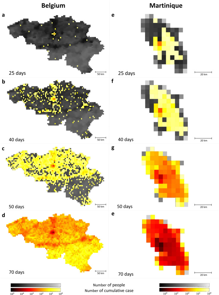
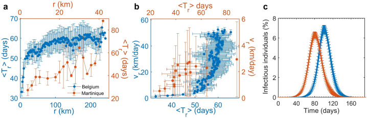
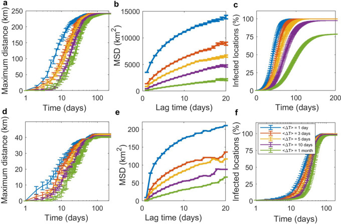
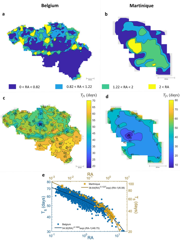
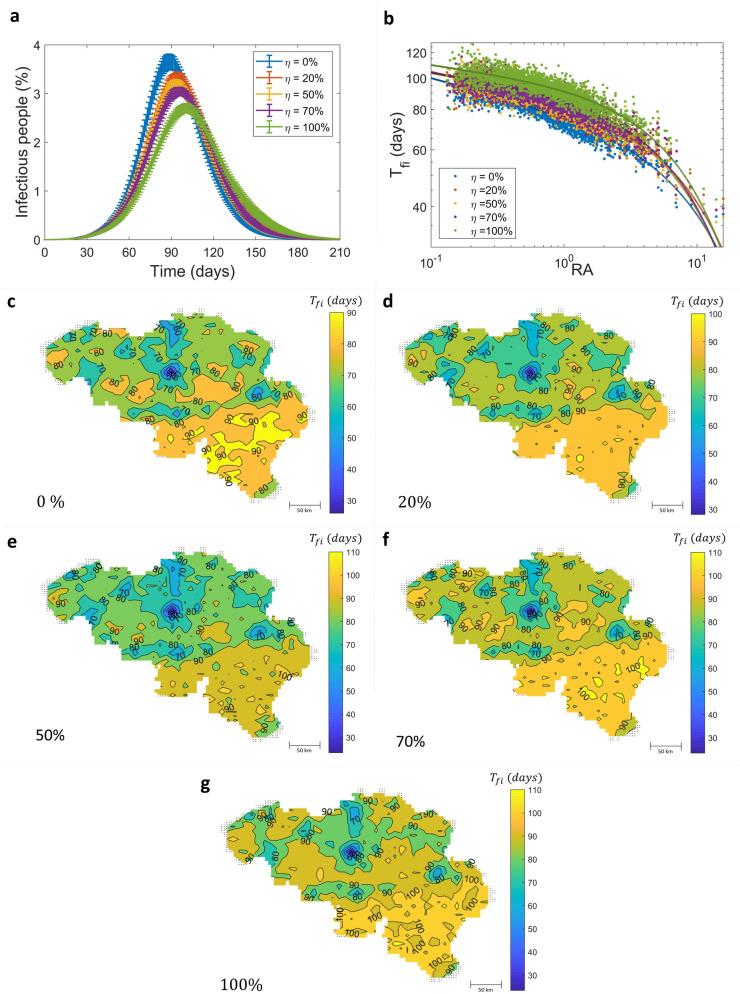
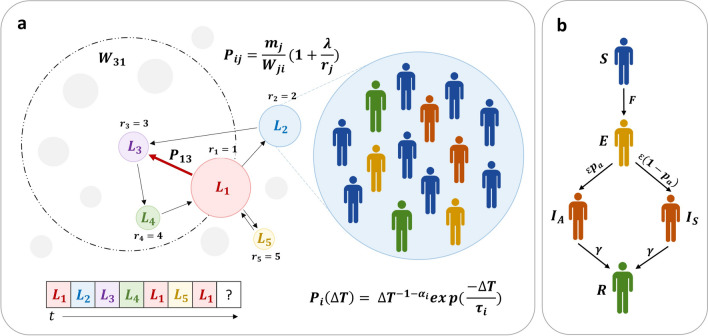
Human mobility plays a crucial role in the temporal and spatial spreading of infectious diseases. During the past few decades, researchers have been extensively investigating how human mobility affects the propagation of diseases. However, the mechanism of human mobility shaping the spread of epidemics is still elusive. Here we examined the impact of human mobility on the infectious disease spread by developing the individual-based SEIR model that incorporates a model of human mobility. We considered the spread of human influenza in two contrasting countries, namely, Belgium and Martinique, as case studies, to assess the specific roles of human mobility on infection propagation. We found that our model can provide a geo-temporal spreading pattern of the epidemics that cannot be captured by a traditional homogenous epidemic model. The disease has a tendency to jump to high populated urban areas before spreading to more rural areas and then subsequently spread to all neighboring locations. This heterogeneous spread of the infection can be captured by the time of the first arrival of the infection [Formula: see text], which relates to the landscape of the human mobility characterized by the relative attractiveness. These findings can provide insights to better understand and forecast the disease spreading.


Conflict of interest statement

The authors declare no competing interests.

Figures

Figure 1
Figure 1
Geotemporal spreading pattern of an uncontrolled epidemic in Belgium and Martinique. The snapshots show a spreading pattern of an epidemic in Belgium (left column) and Martinique (right column) with R0 = 1.9 at 25, 40, 50, and 70 days after the introduction of the disease. The shade of grey represents the population density, and the shade of red indicates the cumulative number of infected individuals in each location. Population sizes simulated for Belgium and Martinique are 1.1×10⁷ within 2,252 locations and 4×10⁵ within 86 locations, respectively. The parameter values used in the simulations are summarized in Table 1 in the Methods section.
Figure 2
Figure 2
Radial speed of disease spread. (a) The radial-averaged time of the first arrival (Tr) of infection in each location at radius r centered at the first infected location for Belgium (blue) and Martinique (red) and (b) the corresponding radial speed of spread. (c) The epidemic curves showing the number of infectious individuals in Belgium (blue) and Martinique (red).
Figure 3
Figure 3
Effects of waiting time on the disease spreading characteristics. (a, d) The maximum distance, which is the distance between the first infected location and the farthest infected location. (b, e) The time-averaged mean square displacement (MSD) of infectious individuals as a function of lag time. (c, f) The cumulative number of infected locations. The top and bottom rows show the simulation results for Belgium (with the population density reduced by 100 times) and Martinique, respectively. The number of simulations for Belgium and Martinique was 50 and 30, respectively.
Figure 4
Figure 4
Relationship of the relative attractiveness of locations (RA) and disease spreading in Belgium and Martinique. (a, b) The maps illustrate the RA of each location in Belgium and Martinique, respectively. Each section represents the different RA with different colors. (c, d) The contours show the first arrival time (Tfi) of disease occurrence in each location after the end of epidemics; 6 months. (e) The relationship between RA and Tfi of Belgium (blue) and Martinique (red) are fitted by the truncated power law.
Figure 5
Figure 5
Effectiveness of symptomatic infectious individual movement restriction in Belgium. (a) The numbers of infectious individuals. (b) The relationship between RA and Tfi. Symbols indicate the results obtained from the model simulations. Lines correspond to the truncated power-law equation. (cg) Contours showing the first arrival time of disease occurrence in each location with a different percentage of infectious individuals which are banned from travelling to other locations (η); 0%, 20%, 50%, 70%, and 100%, respectively.
Figure 6
Figure 6
Schematic illustration of the epidemic model incorporating individual human mobility. (a) Five visited locations, for example, are denoted by letters L1-L5 with different colors. The population density of a location is proportional to the size of the circle that contains the letter. An example of a sequence of letters indicating the individual’s movement trajectory, L1L2L3L4L5L1 , is shown at the bottom. The transition probability for an individual moving from location i to location j is governed by two elements, namely, a gravity-like part (Bij=mj/Wji) and a memory effect Aj=1+λ/rj. If location j has never been visited before (grey circle), its Aj value is assumed to be unity, Aj=1; thus, it will be visited with pij=mj/Wji. For the previously visited location j, it can be visited again with pij=mjWji1+λrj, where rj is an index indicating that location j is the rth visited location. At a certain time, each location contains a number of human individuals who will stay at the location for different periods of time drawn from the waiting time distribution PΔT. The figure was adapted from the model proposed by Yan et al.. (b) Based on the individual’s disease transmission dynamics, individuals are categorized into five compartments, namely, the susceptible (S), exposed (E), asymptomatic infectious (IA), symptomatic infectious (Is), and recovered (R) compartments. Individuals in the exposed compartment move to the asymptomatic infectious compartment with the probability pa.

References

    1. Jones KE, et al. Global trends in emerging infectious diseases. Nature. 2008;451(7181):990. - PMC - PubMed
    1. Bloom DE, Cadarette D. Infectious disease threats in the 21st century: strengthening the global response. Front. Immunol. 2019;10:549. - PMC - PubMed
    1. Altizer S, et al. Seasonality and the dynamics of infectious diseases. Ecol. Lett. 2006;9(4):467–484. - PubMed
    1. Mossong J, et al. Social contacts and mixing patterns relevant to the spread of infectious diseases. PLoS Med. 2008;5(3):e74. - PMC - PubMed
    1. Dushoff J, Levin S. The effects of population heterogeneity on disease invasion. Math. Biosci. 1995;128(1–2):25–40. - PubMed

Publication types

Cite

AltStyle によって変換されたページ (->オリジナル) /