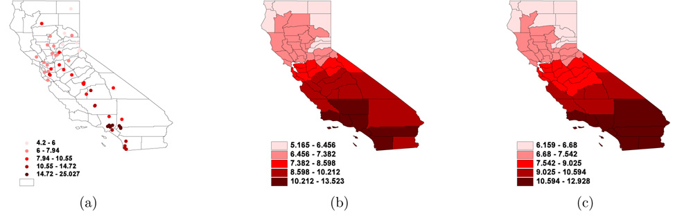
Gaussian geostatistical models (GGMs) and Gaussian Markov random fields (GM-RFs) are two distinct approaches commonly used in spatial models for modeling point referenced and areal data, respectively. In this paper, the relations between GGMs and GMRFs are explored based on approximations of GMRFs by GGMs, and approximations of GGMs by GMRFs. Two new metrics of approximation are proposed: (i) the Kullback-Leibler discrepancy of spectral densities and (ii) the chi-squared distance between spectral densities. The distances between the spectral density functions of GGMs and GMRFs measured by these metrics are minimized to obtain the approximations of GGMs and GMRFs. The proposed methodologies are validated through several empirical studies. We compare the performance of our approach to other methods based on covariance functions, in terms of the average mean squared prediction error and also the computational time. A spatial analysis of a dataset on PM(2.5) collected in California is presented to illustrate the proposed method.

• R01 ES014843/ES/NIEHS NIH HHS/United States

References

-
- Arfken G, Weber HJ. Mathematical Methods for Physicists. 4th ed. San Diego, California: Academic Press; 1995.
- Besag J. Spatial interaction and the statistical analysis of lattice systems. Journal of the Royal Statistical Society. 1974;36:192–236.
- Besag J. On a system of two-dimensional recurrence equations. Journal of the Royal Statistical Society. 1981;43:302–309.
- Besag J, Kooperberg C. On conditional and intrinsic autoregressions. Biometrika. 1995;82:733–746.
- Besag J, York JC, Mollie A. Bayesian image restoration, with two applications in spatial statistics (with discussion) Annals of the Institute of Statistical Mathematics. 1991;43:1–59.
Grants and funding
LinkOut - more resources
Full Text Sources