Division of Mathematical and Physical Sciences, Kanazawa University, Kanazawa 920-1192, Japan
Department of Mathematics, University of Rajshahi, Rajshahi 6205, Bangladesh
Japan Science and Technology Agency, PRESTO, Kawaguchi 332-0012, Japan
* Corresponding author: Md. Masum Murshed
* Corresponding author: Md. Masum MurshedEnergy estimates of the shallow water equations (SWEs) with a transmission boundary condition are studied theoretically and numerically. In the theoretical part, using a suitable energy, we begin with deriving an equality which implies an energy estimate of the SWEs with the Dirichlet and the slip boundary conditions. For the SWEs with a transmission boundary condition, an inequality for the energy estimate is proved under some assumptions to be satisfied in practical computation. In the numerical part, based on the theoretical results, the energy estimate of the SWEs with a transmission boundary condition is confirmed numerically by a finite difference method (FDM). The choice of a positive constant $ c_0 $ used in the transmission boundary condition is investigated additionally. Furthermore, we present numerical results by a Lagrange-Galerkin scheme, which are similar to those by the FDM. The theoretical results along with the numerical results strongly recommend that the transmission boundary condition is suitable for the boundaries in the open sea.
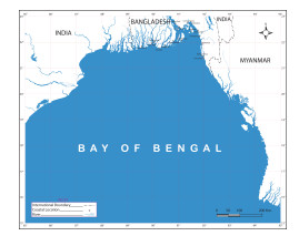
Figure 1. The Bay of Bengal and the coastal region of Bangladesh
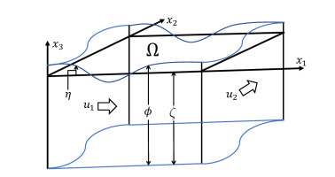
Figure 2. Model domain
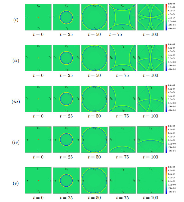
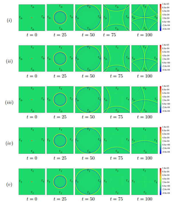
Figure 3. Color contours of $ \eta_h^k $ by finite difference scheme (25) for the five cases $ (i) $-$ (v) $ discussed in Subsection 4.2
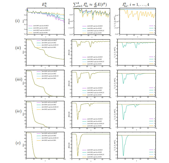
Figure 4. Graphs of $ E_h^k $ (left), $ \sum_{i = 1}^4 I_{hi}^k \approx \frac{d}{dt} E(t) $ (center) and $ I_{hi}^k ,ドル $ i = 1, \ldots, 4 ,ドル (right) versus $ t = t^k\; (\ge 0, k\in \mathbb{Z}) $ for the five cases $ (i) $-$ (v) $
Figure 5. Color contours of $ \eta_h^k $ by Lagrange-Galerkin scheme (26) for the five cases $ (i) $-$ (v) $ discussed in Section 5
Table 1.
Maximum and minimum values of
| $ \varGamma_T $ | $ \varGamma_D $ | $ I_{h1} $ | $ I_{h2} $ | $ I_{h3} $ | $ I_{h4} $ | |
| 0 | 4 | Max | 0.00 | 0.00 | 0.00 | 0.00 |
| Min | 0.00 | 0.00 | 0.00 | $ -8.63 \times 10^{-7} $ | ||
| 1 | 3 | Max | $ 1.10 \times 10^{-4} $ | 0.00 | $ 1.44 \times 10^{-9} $ | 0.00 |
| Min | $ -2.59 \times 10^{-3} $ | $ -3.37 $ | $ -1.25\times 10^{-9} $ | $ -3.76\times 10^{-7} $ | ||
| 2 | 2 | Max | $ 1.86 \times 10^{-4} $ | 0.00 | $ 1.72 \times 10^{-9} $ | 0.00 |
| Min | $ -3.38 \times 10^{-3} $ | -6.27 | $ -2.50 \times 10^{-9} $ | $ -2.31 \times 10^{-7} $ | ||
| 3 | 1 | Max | $ 1.43 \times 10^{-4} $ | 0.00 | $ 2.58 \times 10^{-9} $ | 0.00 |
| Min | $ -5.06 \times 10^{-3} $ | $ -9.40 $ | $ -3.75 \times 10^{-9} $ | $ -1.74 \times 10^{-7} $ | ||
| 4 | 0 | Max | $ 2.87 \times 10^{-4} $ | 0.00 | $ 3.47 \times 10^{-9} $ | 0.00 |
| Min | $ -6.75 \times 10^{-3} $ | $ -12.54 $ | $ -5.01 \times 10^{-9} $ | $ -1.14 \times 10^{-7} $ |
Table 2.
| $ c_0 $ | $ \mathcal{S}_h(c_0) $ | |||||
| Case I | Case II | Case III | Case IV | Case V | Case VI | |
| 0.1 | 12.17 | 8.53 | 8.14 | 5.47 | 44.48 | 44.49 |
| 0.2 | 9.89 | 6.97 | 6.35 | 4.04 | 34.36 | 34.37 |
| 0.3 | 8.84 | 6.24 | 5.52 | 3.35 | 28.74 | 28.75 |
| 0.4 | 8.27 | 5.85 | 5.08 | 2.98 | 25.23 | 25.24 |
| 0.5 | 7.93 | 5.61 | 4.84 | 2.79 | 22.82 | 22.83 |
| 0.6 | 7.71 | 5.46 | 4.71 | 2.69 | 21.05 | 21.06 |
| 0.7 | 7.58 | 5.37 | 4.65 | 2.66 | 19.69 | 19.69 |
| 0.8 | 7.51 | 5.32 | 4.63 | 2.67 | 18.60 | 18.61 |
| 0.9 | 7.4805 | 5.2969 | 4.64 | 2.70 | 17.71 | 17.72 |
| 1.0 | 7.4807 | 5.2977 | 4.68 | 2.76 | 16.98 | 16.98 |
| 1.1 | 7.50 | 5.32 | 4.73 | 2.82 | 16.36 | 16.36 |
| 1.2 | 7.55 | 5.35 | 4.79 | 2.89 | 15.83 | 15.84 |
| 1.5 | 7.75 | 5.49 | 5.02 | 3.12 | 14.66 | 14.66 |
Figures(5)
Tables(2)
HTML views(3720) PDF downloads(378) Cited by(0)
The Bay of Bengal and the coastal region of Bangladesh
Model domain
Color contours of
Graphs of
Color contours of