[Applications] [Matlab/Octave] [Self deconvolution] [Excess noise reduction by denominator addition] [Multiple sequential deconvolution] [Segmented deconvolution] [convdeconv function] [Live Script] [Interactive deconvolution in iSignal]
Fourier deconvolution is
the converse of Fourier convolution
in the sense that division is the converse of multiplication. If
you know that m times x equals
n, where m and n are known
but x is unknown, then x equals n
divided by m. Conversely if you know that m
convoluted with x equals n,
where m and n are known but x
is unknown, then x equals m deconvoluted
from n.
In practice, the deconvolution of one signal from another is
usually performed by point-by-point division of the two
signals in the Fourier domain, that is, dividing the Fourier
transforms of the two signals point-by-point and then
inverse-transforming the result. Fourier transforms are usually
expressed in terms of complex numbers, with real and imaginary
parts representing the sine and cosine parts. If the Fourier
transform of the first signal is a + ib, and the Fourier
transform of the second signal is c + id, then the ratio
of the two Fourier transforms is
by the rules for the division
of
complex numbers. Many computer languages will perform this
operation automatically when the two quantities divided are
complex.
Note: The word "deconvolution"
can have two meanings, which can lead to confusion. The Oxford
dictionary defines it as "A process of resolving something into
its constituent elements or removing complication in order to
clarify it", which in one sense applies to Fourier deconvolution.
But the same word is also sometimes used for the process of
resolving or decomposing a set of overlapping peaks into their
separate additive components by the technique of iterative least-squares curve fitting
of a proposed peak model to the data set. However, that process is
actually conceptually distinct from Fourier deconvolution,
because in Fourier deconvolution, the underlying peak shape is
unknown but the broadening function is assumed to be known;
whereas in iterative least-squares curve fitting it's just the
reverse: the peak shape must be known but the width of the
broadening process, which determines the width and shape of the
peaks in the recorded data, is unknown. Thus the term "spectral
deconvolution" is ambiguous: it might mean the Fourier
deconvolution of a response function from a spectrum, or it might
mean the decomposing of a spectrum into its separate additive peak
components. These are different processes; don't get them
confused.
The practical
significance of Fourier deconvolution in signal processing
is that it can be used as a computational way to reverse the
result of a convolution occurring in the physical domain, for
example, to reverse the signal distortion effect of an electrical
filter or of the finite resolution of a spectrometer. In some
cases the physical convolution can be measured experimentally by
applying a single spike impulse ("delta") function to the input of
the system, then that data used as a deconvolution vector.
Deconvolution can also be used to determine the form of a
convolution operation that has been previously applied to a
signal, by deconvoluting the original and the convoluted signals.
These two types of application of Fourier deconvolution are shown
in the two figures below.
Fourier deconvolution is used here to remove the distorting influence of an exponential tailing response function from a recorded signal (Window 1, top left) that is the result of an unavoidable RC low-pass filter action in the electronics. The response function (Window 2, top right) must be known and is usually either calculated on the basis of some theoretical model or is measured experimentally as the output signal produced by applying an impulse (delta) function to the input of the system. The response function, with its maximum at x=0, is deconvoluted from the original signal . The result (bottom, center) shows a closer approximation to the real shape of the peaks; however, the signal-to-noise ratio is unavoidably degraded compared to the recorded signal, because the Fourier deconvolution operation is simply recovering the original signal before the low-pass filtering, noise and all. (Matlab/Octave script)
Note that this process has an effect that is visually similar to resolution enhancement, although the later is done without specific knowledge of the broadening function that caused the peaks to overlap.
A different application of Fourier deconvolution is to reveal the nature of an unknown data transformation function that has been applied to a data set by the measurement instrument itself. In this example, the figure in the top left is a uv-visible absorption spectrum recorded from a commercial photodiode array spectrometer (X-axis: nanometers; Y-axis: milliabsorbance). The figure in the top right is the first derivative of this spectrum produced by an (unknown) algorithm in the software supplied with the spectrometer. The objective here is to understand the nature of the differentiation/smoothing algorithm that the instrument's software uses. The signal in the bottom left is the result of deconvoluting the derivative spectrum (top right) from the original spectrum (top left). This therefore must be the convolution function used by the differentiation algorithm in the spectrometer's software. Rotating and expanding it on the x-axis makes the function easier to see (bottom right). Expressed in terms of the smallest whole numbers, the convolution series is seen to be +2, +1, 0, -1, -2. This simple example of "reverse engineering" would make it easier to compare results from other instruments or to duplicate these result on other equipment.
When applying Fourier
deconvolution to experimental data, for example to remove the
effect of a known broadening or low-pass filter operator caused by
the experimental system, there are four serious problems that
limit the utility of the method:
(1) the convolution occurring in the physical domain might not be accurately modeled by a mathematical convolution;
(2) the width of the convolution - for example the time constant of a low-pass filter operator or the shape and width of a spectrometer slit function - must be known, or at least adjusted by the user to get the best results;
(3) a serious signal-to-noise degradation commonly occurs; any noise added to the signal by the system after the convolution by the broadening or low-pass filter operator will be greatly amplified when the Fourier transform of the signal is divided by the Fourier transform of the broadening operator, because the high frequency components of the broadening operator (the denominator in the division of the Fourier transforms) are typically very small, with some individual components often of the order of 10-12 or 10-15, resulting a huge amplification of those particular frequencies in the resulting deconvoluted signal, which is called "ringing". (See the Matlab/Octave code example at the bottom of this page). The problem can be reduced either by low-pass filtering (smoothing). Smoothing or filtering reduces the amplitude of the highest-frequency components.
You can see the amplification of high frequency noise happening in the example in the first example above. On the other hand, this effect is not observed in the second example, because in that case the noise was present in the original signal, before the convolution performed by the spectrometer's derivative algorithm. The high frequency components of the denominator in the division of the Fourier transforms are typically much larger than in the previous example, avoiding the noise amplification and divide-by-zero errors, and the only post-convolution noise comes from numerical round-off errors in the math computations performed by the derivative and smoothing operation, which is always much smaller than the noise in the original experimental signal.
In many cases, the width of the physical convolution is not known
exactly, so the deconvolution must be adjusted empirically to
yield the best results. Similarly, the width of the final smooth
operation must also be adjusted for best results. The result will
seldom be perfect, especially if the original signal is noisy, but
it is often a better approximation to the real underlying signal
than the recorded data without deconvolution.
As a method for peak sharpening, deconvolution can be
compared to the derivative
peak sharpening method described earlier or to the power method, in
which the raw signal is simply raised to some positive power n.
Matlab
and Octave have a built-in function for Fourier
deconvolution: deconv. An example
of its application is shown below: the vector yc (line 6)
represents a noisy rectangular pulse (y) convoluted with a
transfer function c before being measured. In line 7, c
is deconvoluted from yc, in an attempt to recover the
original y. This requires that the transfer function c
be known. The rectangular signal pulse is recovered in the lower
right (ydc), complete with the noise that was present in
the original signal. The Fourier deconvolution reverses not
only the signal-distorting effect of the convolution by the
exponential function, but also its low-pass noise-filtering
effect. As explained above, there is significant amplification of
any noise that is added after the convolution by the
transfer function (line 5). This script demonstrates that there is
a big difference between noise added before the
convolution (line 3), which is recovered unmodified by the Fourier
deconvolution along with the signal, and noise added after
the convolution (line 6), which is amplified compared to that in
the original signal. Execution time: 0.03 seconds in Matlab; 0.3
seconds in Octave. Download this
script.
x=0:.01:20;
y=zeros(size(x));
% Create a rectangular function y, 200 points wide
y(900:1100)=1;
%
Noise added before
the convolution
y=y+.01.*randn(size(y));
% exponential trailing
convolution function, c
c=exp(-(1:length(y))./30);
% Create exponential trailing rectangular
% function, yc
yc=conv(y,c,'full')./sum(c);
%
Optional noise added after the convolution
%
yc=yc+.01.*randn(size(yc));
% Attempt to recover y by deconvoluting c from yc
ydc=deconv(yc,c).*sum(c);
% The sum(c2) is included simply to scale
the
% amplitude of the result to match the original y.
% Plot all the steps in separate subplots
subplot(2,2,1); plot(x,y); title('original y');
subplot(2,2,2); plot(x,c);title('c'); subplot(2,2,3);
plot(x,yc(1:2001)); title('yc'); subplot(2,2,4);
plot(x,ydc);title('recovered y')
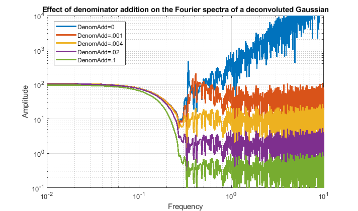
(a) The left-hand
(low frequency) side is a smooth curved region, which are the
signal components of the deconvoluted signal. The narrower the
signal peak, the more gradually the curve drops off at higher
frequencies.
(b) The right-hand (high frequency) end of the spectrum is
dominated by the noise and ringing in the deconvoluted signal.
Observing
these spectra can be a useful guide to adjusting the
deconvolution width and the noise filtering. You can see that,
in this particular case, the noise has caused a pronounced spike
near the middle of the spectrum, which is the cause of the
oscillatory ringing in the peak plots. As the cutoff frequency
is decreased, the high-frequency components are reduced, as
expected, but the spike still remains even at the lowest
cutoff (green line), at which point the width of the
deconvoluted peak has been broadened by the filter,
counteracting the original intent of deconvolution.
This
problem can be solved by an independent method of noise
reduction introduced by Farooq Wahab and myself in 2023
(reference 96). This involves simply adding a
small positive non-zero constant or distribution function to the
denominator in the deconvolution process, which increases the
excessively small high-frequency members in the denominator. The
quantity added is small, typically or 1 to 5 percent of the
amplitude of the denominator. In Matlab, the basic devolution
operation is coded like so:
ydc=ifft(fft(y)./(fft(df))).*sum(df)
Here is the code for the case where the denominator addition is a constant:
D=fft(df)+DA.*max(fft(df));
ydcDA=ifft(fft(y)./D).*sum(df);
where y is the original signal, D is the denominator, df is the deconvolution function and FDA is the fractional denominator addition. The addition is scaled to the maximum value of the fft of the deconvolution function df so that the quantity added will adjust to the varying amplitudes of different experimental signals.
An alternative is to add a constant only to those members of the denominator below a specified threshold, e.g. using the "no lower than" function nlt(a,b) :
D=nlt(fftc,FDA.*0.01.*max(fftc));
ydcDA=ifft(fft(y)./D).*sum(df);
Graphical user interface, diagramDescription automatically generated ChartDescription automatically generated
Deconvolution for peak area measurements. Measuring the areas under peaks is a common requirement in quantitative analysis, but it works only if there is sufficient separation between peaks. Because deconvolution sharpens peaks but does not change the area under them, it can be used to improve the measurement of the areas of overlapping peaks. In the Matlab script GLSDPerpDropDemo16.m , the areas of a group of three partially overlapping peaks is measured, by the perpendicular drop method, before and after peak sharpening by Fourier self-deconvolution. The measurements are repeated with random peak height, to test how the peak overlap interferes with precise area measurement. After sixteen trials with randomized peak heights, the true peak area are plotted against the measured areas, and the R2 values for each case are compared before and after deconvolution. The results are summarized on this PDF file. Conclusion: in every case, from the "easiest" to the most challenging, deconvolution yields the best results.
Self-deconvolution
sharpening of the IR spectrum of Heptene, 'HepteneTestData.csv'
In iSignal version 8.3 , and its Octave
version, the downloadable interactive multipurpose
signal processing Matlab function, you can press Shift-V to
display the menu
of
Fourier convolution and deconvolution operations that allow you to convolute or to
deconvolute a Gaussian, Lorentzian or exponential function. It
will ask you for the initial width or time constant of
the deconvolution function (Vwidth, in X units), then you
can use the 3 and 4 keys
to decrease or increase the width by 10% (or Shift-3 and Shift-4 to
adjust
by 1%).Here's an application to a real
experimental signal. The denominator addition (to suppress
ringing and noise) is controlled by the 5
and 6 keys.