• Home
• >
• Tutorial
• >
• Head Pose Estimation using OpenCV and Dlib

• Satya Mallick
• on September 26, 2016

Head Pose Estimation using OpenCV and Dlib

In this tutorial we will learn how to estimate the pose of a human head in a photo using OpenCV and Dlib. In many applications, we need to know how the head is tilted with respect to a camera. In a virtual reality application, for example, one can use the

• Tutorial

In this tutorial we will learn how to estimate the pose of a human head in a photo using OpenCV and Dlib.

In many applications, we need to know how the head is tilted with respect to a camera. In a virtual reality application, for example, one can use the pose of the head to render the right view of the scene. In a driver assistance system, a camera looking at a driver’s face in a vehicle can use head pose estimation to see if the driver is paying attention to the road. And of course one can use head pose based gestures to control a hands-free application / game. For example, yawing your head left to right can signify a NO. But if you are from southern India, it can signify a YES! To understand the full repertoire of head pose based gestures used by my fellow Indians, please partake in the hilarious video below.

My point is that estimating the head pose is useful. Sometimes.

Before proceeding with the tutorial, I want to point out that this post belongs to a series I have written on face processing. Some of the articles below are useful in understanding this post and others complement it.

1. Facial Landmark Detection
2. Face Swap
3. Face Averaging
4. Face Morphing

What is pose estimation ?

In computer vision the pose of an object refers to its relative orientation and position with respect to a camera. You can change the pose by either moving the object with respect to the camera, or the camera with respect to the object.

The pose estimation problem described in this tutorial is often referred to as Perspective-n-Point problem or PNP in computer vision jargon. As we shall see in the following sections in more detail, in this problem the goal is to find the pose of an object when we have a calibrated camera, and we know the locations of n 3D points on the object and the corresponding 2D projections in the image.

How to mathematically represent camera motion ?

A 3D rigid object has only two kinds of motions with respect to a camera.

1. Translation : Moving the camera from its current 3D location (X, Y, Z) to a new 3D location (X', Y', Z') is called translation. As you can see translation has 3 degrees of freedom — you can move in the X, Y or Z direction. Translation is represented by a vector \mathbf{t} which is equal to ( X' - X, Y' - Y, Z' - Z ).
2. Rotation : You can also rotate the camera about the X, Y and Z axes. A rotation, therefore, also has three degrees of freedom. There are many ways of representing rotation. You can represent it using Euler angles ( roll, pitch and yaw ), a 3\times3 rotation matrix, or a direction of rotation (i.e. axis ) and angle.

So, estimating the pose of a 3D object means finding 6 numbers — three for translation and three for rotation.

What do you need for pose estimation ?

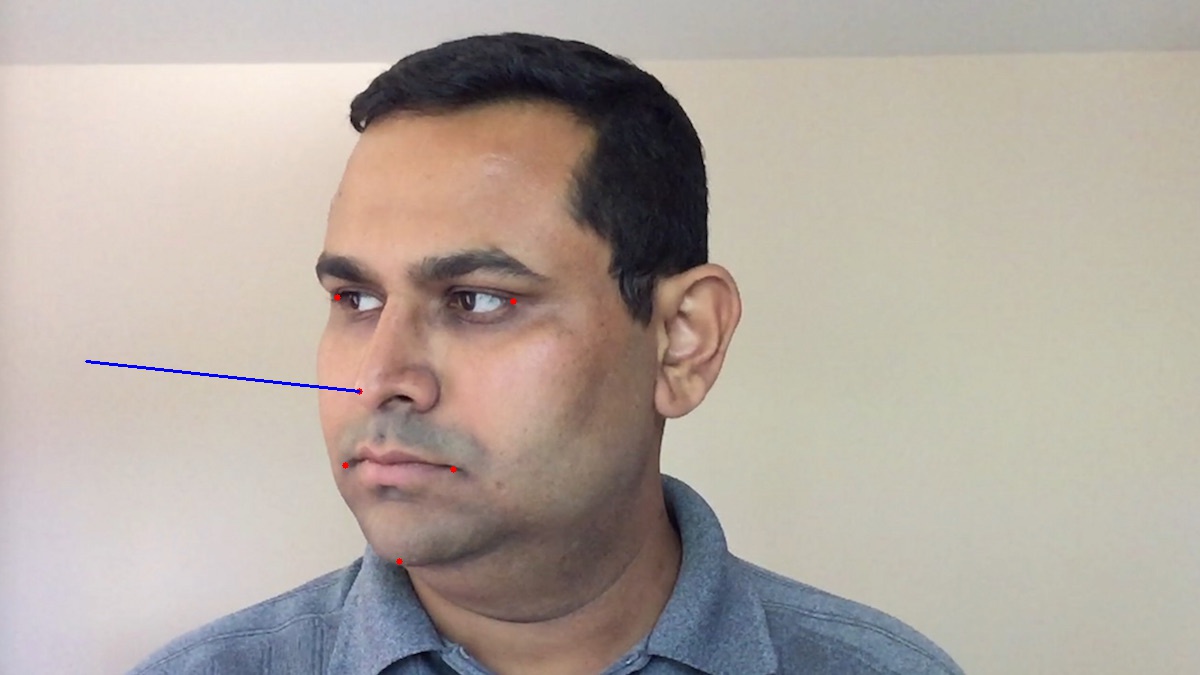
To calculate the 3D pose of an object in an image you need the following information

1. 2D coordinates of a few points : You need the 2D (x,y) locations of a few points in the image. In the case of a face, you could choose the corners of the eyes, the tip of the nose, corners of the mouth etc. Dlib’s facial landmark detector provides us with many points to choose from. In this tutorial, we will use the tip of the nose, the chin, the left corner of the left eye, the right corner of the right eye, the left corner of the mouth, and the right corner of the mouth.
2. 3D locations of the same points : You also need the 3D location of the 2D feature points. You might be thinking that you need a 3D model of the person in the photo to get the 3D locations. Ideally yes, but in practice, you don’t. A generic 3D model will suffice. Where do you get a 3D model of a head from ? Well, you really don’t need a full 3D model. You just need the 3D locations of a few points in some arbitrary reference frame. In this tutorial, we are going to use the following 3D points.
   1. Tip of the nose : ( 0.0, 0.0, 0.0)
   2. Chin : ( 0.0, -330.0, -65.0)
   3. Left corner of the left eye : (-225.0f, 170.0f, -135.0)
   4. Right corner of the right eye : ( 225.0, 170.0, -135.0)
   5. Left corner of the mouth : (-150.0, -150.0, -125.0)
   6. Right corner of the mouth : (150.0, -150.0, -125.0)

      Note that the above points are in some arbitrary reference frame / coordinate system. This is called the World Coordinates ( a.k.a Model Coordinates in OpenCV docs ) .

3. Intrinsic parameters of the camera. As mentioned before, in this problem the camera is assumed to be calibrated. In other words, you need to know the focal length of the camera, the optical center in the image and the radial distortion parameters. So you need to calibrate your camera. Of course, for the lazy dudes and dudettes among us, this is too much work. Can I supply a hack ? Of course, I can! We are already in approximation land by not using an accurate 3D model. We can approximate the optical center by the center of the image, approximate the focal length by the width of the image in pixels and assume that radial distortion does not exist. Boom! you did not even have to get up from your couch!

How do pose estimation algorithms work ?

There are several algorithms for pose estimation. The first known algorithm dates back to 1841. It is beyond the scope of this post to explain the details of these algorithms but here is a general idea.

There are three coordinate systems in play here. The 3D coordinates of the various facial features shown above are in world coordinates. If we knew the rotation and translation ( i.e. pose ), we could transform the 3D points in world coordinates to 3D points in camera coordinates. The 3D points in camera coordinates can be projected onto the image plane ( i.e. image coordinate system ) using the intrinsic parameters of the camera ( focal length, optical center etc. ).

Let’s dive into the image formation equation to understand how these above coordinate systems work. In the figure above, o is the center of the camera and plane shown in the figure is the image plane. We are interested in finding out what equations govern the projection p of the 3D point P onto the image plane.

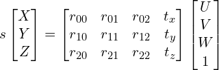
Let’s assume we know the location ( U, V, W ) of a 3D point P in World Coordinates. If we know the rotation \mathbf{R} ( a 3×3 matrix ) and translation \mathbf{t} ( a 3×1 vector ), of the world coordinates with respect to the camera coordinates, we can calculate the location (X, Y, Z) of the point P in the camera coordinate system using the following equation.

(1) [画像:\begin{align*}\begin{bmatrix} X \\ Y \\ Z \end{bmatrix} &= \mathbf{R} \begin{bmatrix}U \\ V \\ W \end{bmatrix} + \mathbf{t} \\\Rightarrow \begin{bmatrix} X \\ Y \\ Z \end{bmatrix} &= \left [ \mathbf{R} \enspace | \enspace \mathbf{t} \right ] \begin{bmatrix}U \\ V \\ W \\ 1 \end{bmatrix}\end{align*}]

In expanded form, the above equation looks like this

(2) [画像:\begin{align*}\begin{bmatrix} X \\ Y \\ Z \end{bmatrix} =\begin{bmatrix}r_{00} & r_{01} & r_{02} & t_{x}\\r_{10} & r_{11} & r_{12} & t_{y}\\r_{20} & r_{21} & r_{22} & t_{z}\\\end{bmatrix} \begin{bmatrix}U \\ V \\ W \\ 1 \end{bmatrix}\end{align*}]

If you have ever taken a Linear Algebra class, you will recognize that if we knew sufficient number of point correspondences ( i.e. (X, Y, Z) and (U, V, W) ), the above is a linear system of equations where the r_{ij} and (t_x, t_y, t_z) are unknowns and you can trivially solve for the unknowns.

As you will see in the next section, we know (X, Y, Z) only up to an unknown scale, and so we do not have a simple linear system.

Direct Linear Transform

We do know many points on the 3D model ( i.e. (U, V, W) ), but we do not know (X, Y, Z). We only know the location of the 2D points ( i.e. (x, y) ). In the absence of radial distortion, the coordinates (x, y) of point p in the image coordinates is given by

(3) [画像:\begin{align*}\begin{bmatrix} x \\ y \\ 1 \end{bmatrix} &=s \begin{bmatrix} f_x & 0 & c_x \\ 0 & f_y & c_y \\ 0 & 0 & 1 \end{bmatrix}\begin{bmatrix} X \\ Y \\ Z \end{bmatrix}\end{align*}]

where, f_x and f_y are the focal lengths in the x and y directions, and (c_x, c_y) is the optical center. Things get slightly more complicated when radial distortion is involved and for the purpose of simplicity I am leaving it out.

What about that s in the equation ? It is an unknown scale factor. It exists in the equation due to the fact that in any image we do not know the depth. If you join any point P in 3D to the center o of the camera, the point p, where the ray intersects the image plane is the image of P. Note that all the points along the ray joining the center of the camera and point P produce the same image. In other words, using the above equation, you can only obtain (X, Y, Z) up to a scale s.

Now this messes up equation 2 because it is no longer the nice linear equation we know how to solve. Our equation looks more like

(4) [画像:\begin{align*}s \begin{bmatrix} X \\ Y \\ Z \end{bmatrix} =\begin{bmatrix}r_{00} & r_{01} & r_{02} & t_{x}\\r_{10} & r_{11} & r_{12} & t_{y}\\r_{20} & r_{21} & r_{22} & t_{z}\\\end{bmatrix} \begin{bmatrix}U \\ V \\ W \\ 1 \end{bmatrix}\end{align*}]

Fortunately, the equation of the above form can be solved using some algebraic wizardry using a method called Direct Linear Transform (DLT). You can use DLT any time you find a problem where the equation is almost linear but is off by an unknown scale.

Levenberg-Marquardt Optimization

The DLT solution mentioned above is not very accurate because of the following reasons . First, rotation \mathbf{R} has three degrees of freedom but the matrix representation used in the DLT solution has 9 numbers. There is nothing in the DLT solution that forces the estimated 3×3 matrix to be a rotation matrix. More importantly, the DLT solution does not minimize the correct objective function. Ideally, we want to minimize the reprojection error that is described below.

As shown in the equations 2 and 3, if we knew the right pose ( \mathbf{R} and \mathbf{t} ), we could predict the 2D locations of the 3D facial points on the image by projecting the 3D points onto the 2D image. In other words, if we knew \mathbf{R} and \mathbf{t} we could find the point p in the image for every 3D point P.

We also know the 2D facial feature points ( using Dlib or manual clicks ). We can look at the distance between projected 3D points and 2D facial features. When the estimated pose is perfect, the 3D points projected onto the image plane will line up almost perfectly with the 2D facial features. When the pose estimate is incorrect, we can calculate a re-projection error measure — the sum of squared distances between the projected 3D points and 2D facial feature points.

As mentioned earlier, an approximate estimate of the pose ( \mathbf{R} and \mathbf{t} ) can be found using the DLT solution. A naive way to improve the DLT solution would be to randomly change the pose ( \mathbf{R} and \mathbf{t} ) slightly and check if the reprojection error decreases. If it does, we can accept the new estimate of the pose. We can keep perturbing \mathbf{R} and \mathbf{t} again and again to find better estimates. While this procedure will work, it will be very slow. Turns out there are principled ways to iteratively change the values of \mathbf{R} and \mathbf{t} so that the reprojection error decreases. One such method is called Levenberg-Marquardt optimization. Check out more details on Wikipedia.

OpenCV solvePnP

In OpenCV the function solvePnP and solvePnPRansac can be used to estimate pose.

solvePnP implements several algorithms for pose estimation which can be selected using the parameter flag. By default it uses the flag SOLVEPNP_ITERATIVE which is essentially the DLT solution followed by Levenberg-Marquardt optimization. SOLVEPNP_P3P uses only 3 points for calculating the pose and it should be used only when using solvePnPRansac.

In OpenCV 3, two new methods have been introduced — SOLVEPNP_DLS and SOLVEPNP_UPNP. The interesting thing about SOLVEPNP_UPNP is that it tries to estimate camera internal parameters also.

OpenCV solvePnPRansac

solvePnPRansac is very similar to solvePnP except that it uses Random Sample Consensus ( RANSAC ) for robustly estimating the pose.

Using RANSAC is useful when you suspect that a few data points are extremely noisy. For example, consider the problem of fitting a line to 2D points. This problem can be solved using linear least squares where the distance of all points from the fitted line is minimized. Now consider one bad data point that is wildly off. This one data point can dominate the least squares solution and our estimate of the line would be very wrong. In RANSAC, the parameters are estimated by randomly selecting the minimum number of points required. In a line fitting problem, we randomly select two points from all data and find the line passing through them. Other data points that are close enough to the line are called inliers. Several estimates of the line are obtained by randomly selecting two points, and the line with the maximum number of inliers is chosen as the correct estimate.

The usage of solvePnPRansac is shown below and parameters specific to solvePnPRansac are explained.

OpenCV POSIT

OpenCV used to a pose estimation algorithm called POSIT. It is still present in the C API ( cvPosit ), but is not part of the C++ API. POSIT assumes a scaled orthographic camera model and therefore you do not need to supply a focal length estimate. This function is now obsolete and I would recommend using one of the algorithms implemented in solvePnp.

OpenCV Pose Estimation Code : C++ / Python

In this section, I have shared example code in C++ and Python for head pose estimation in a single image. You can download the image headPose.jpg here.

The locations of facial feature points are hard coded and if you want to use your own image, you will need to change the vector image_points

C++

#include <opencv2/opencv.hpp>
using namespace std;
using namespace cv;
int main(int argc, char **argv)
{
 // Read input image
 cv::Mat im = cv::imread("headPose.jpg");
 // 2D image points. If you change the image, you need to change vector
 std::vector<cv::Point2d> image_points;
 image_points.push_back( cv::Point2d(359, 391) ); // Nose tip
 image_points.push_back( cv::Point2d(399, 561) ); // Chin
 image_points.push_back( cv::Point2d(337, 297) ); // Left eye left corner
 image_points.push_back( cv::Point2d(513, 301) ); // Right eye right corner
 image_points.push_back( cv::Point2d(345, 465) ); // Left Mouth corner
 image_points.push_back( cv::Point2d(453, 469) ); // Right mouth corner
 // 3D model points.
 std::vector<cv::Point3d> model_points;
 model_points.push_back(cv::Point3d(0.0f, 0.0f, 0.0f)); // Nose tip
 model_points.push_back(cv::Point3d(0.0f, -330.0f, -65.0f)); // Chin
 model_points.push_back(cv::Point3d(-225.0f, 170.0f, -135.0f)); // Left eye left corner
 model_points.push_back(cv::Point3d(225.0f, 170.0f, -135.0f)); // Right eye right corner
 model_points.push_back(cv::Point3d(-150.0f, -150.0f, -125.0f)); // Left Mouth corner
 model_points.push_back(cv::Point3d(150.0f, -150.0f, -125.0f)); // Right mouth corner
 // Camera internals
 double focal_length = im.cols; // Approximate focal length.
 Point2d center = cv::Point2d(im.cols/2,im.rows/2);
 cv::Mat camera_matrix = (cv::Mat_<double>(3,3) << focal_length, 0, center.x, 0 , focal_length, center.y, 0, 0, 1);
 cv::Mat dist_coeffs = cv::Mat::zeros(4,1,cv::DataType<double>::type); // Assuming no lens distortion
 cout << "Camera Matrix " << endl << camera_matrix << endl ;
 // Output rotation and translation
 cv::Mat rotation_vector; // Rotation in axis-angle form
 cv::Mat translation_vector;
 // Solve for pose
 cv::solvePnP(model_points, image_points, camera_matrix, dist_coeffs, rotation_vector, translation_vector);
 // Project a 3D point (0, 0, 1000.0) onto the image plane.
 // We use this to draw a line sticking out of the nose
 vector<Point3d> nose_end_point3D;
 vector<Point2d> nose_end_point2D;
 nose_end_point3D.push_back(Point3d(0,0,1000.0));
 projectPoints(nose_end_point3D, rotation_vector, translation_vector, camera_matrix, dist_coeffs, nose_end_point2D);
 for(int i=0; i < image_points.size(); i++)
 {
 circle(im, image_points[i], 3, Scalar(0,0,255), -1);
 }
 cv::line(im,image_points[0], nose_end_point2D[0], cv::Scalar(255,0,0), 2);
 cout << "Rotation Vector " << endl << rotation_vector << endl;
 cout << "Translation Vector" << endl << translation_vector << endl;
 cout << nose_end_point2D << endl;
 // Display image.
 cv::imshow("Output", im);
 cv::waitKey(0);
}

Python

#!/usr/bin/env python
import cv2
import numpy as np
# Read Image
im = cv2.imread("headPose.jpg");
size = im.shape
#2D image points. If you change the image, you need to change vector
image_points = np.array([
 (359, 391), # Nose tip
 (399, 561), # Chin
 (337, 297), # Left eye left corner
 (513, 301), # Right eye right corne
 (345, 465), # Left Mouth corner
 (453, 469) # Right mouth corner
 ], dtype="double")
# 3D model points.
model_points = np.array([
 (0.0, 0.0, 0.0), # Nose tip
 (0.0, -330.0, -65.0), # Chin
 (-225.0, 170.0, -135.0), # Left eye left corner
 (225.0, 170.0, -135.0), # Right eye right corne
 (-150.0, -150.0, -125.0), # Left Mouth corner
 (150.0, -150.0, -125.0) # Right mouth corner
 ])
# Camera internals
focal_length = size[1]
center = (size[1]/2, size[0]/2)
camera_matrix = np.array(
 [[focal_length, 0, center[0]],
 [0, focal_length, center[1]],
 [0, 0, 1]], dtype = "double"
 )
print "Camera Matrix :\n {0}".format(camera_matrix)
dist_coeffs = np.zeros((4,1)) # Assuming no lens distortion
(success, rotation_vector, translation_vector) = cv2.solvePnP(model_points, image_points, camera_matrix, dist_coeffs, flags=cv2.CV_ITERATIVE)
print "Rotation Vector:\n {0}".format(rotation_vector)
print "Translation Vector:\n {0}".format(translation_vector)
# Project a 3D point (0, 0, 1000.0) onto the image plane.
# We use this to draw a line sticking out of the nose
(nose_end_point2D, jacobian) = cv2.projectPoints(np.array([(0.0, 0.0, 1000.0)]), rotation_vector, translation_vector, camera_matrix, dist_coeffs)
for p in image_points:
 cv2.circle(im, (int(p[0]), int(p[1])), 3, (0,0,255), -1)
p1 = ( int(image_points[0][0]), int(image_points[0][1]))
p2 = ( int(nose_end_point2D[0][0][0]), int(nose_end_point2D[0][0][1]))
cv2.line(im, p1, p2, (255,0,0), 2)
# Display image
cv2.imshow("Output", im)
cv2.waitKey(0)

Real time pose estimation using Dlib

The video included in this post was made using my fork of dlib which is freely available for subscribers of this blog. If you have already subscribed, please check the welcome email for link to my dlib fork and check out this file

dlib/examples/webcam_head_pose.cpp

If you have not subscribed yet, please do so in the section below

• dlib, Head Pose, OpenCV, Pose, solvepnp, solvepnpransac

Read Next

Subscribe to our Newsletter

Subscribe to our email newsletter to get the latest posts delivered right to your email.