1. Introduction
Emission inventories are important datasets for understanding air quality. Air pollutant emissions are estimated using a bottom-up method, in which fuel consumption, emission factors, and removal efficiency are multiplied. A disadvantage of the bottom-up method is the time lag in compiling the dataset because the method relies on statistical data. Emissions change dramatically due to changes in the economy, regulation, and technology, along with numerous other factors. Therefore, the latest emissions estimates are urgently needed for understanding air quality and for more accurate data to generate chemical transport models. Accurate emissions estimates are particularly important for Asia, where the anthropogenic emissions have already exceded those of Europe and the US (Janssens-Maenhout et al 2015). For example, several episodic events with substantial emission changes in China have been reported, including the Sino-African Summit in November 2006 in Beijing (e.g. Wang et al 2007), the Beijing Olympics in August 2008 (e.g. Mijling et al 2009), the economic recession from late 2008 to mid-2009 (e.g. Lin and McElroy 2011), the Shanghai World Exposition from May to October 2010 (e.g. Hao et al 2011), and the Asia-Pacific Economic Cooperation (APEC) meeting held in Beijing in November 2014 (e.g. Sun et al 2016).
To overcome the disadvantages of bottom-up emission inventories, the main approach is inverse estimation, which optimizes emission inventories based on forward model simulation with observational constraints. Recently, many studies have proposed inverse estimation with advanced data assimilation techniques, including four-dimensional variational assimilation (4D-Var) (Müller and Stavrakou 2005, Yumimoto and Uno 2006, Kurokawa et al 2009), and ensemble Kalman Filter (Yumimoto and Takemura 2011, Miyazaki and Eskes 2013, Miyazaki et al 2015, 2017). We previously estimated Chinese CO emissions based on a combination of Green’s function method with the tagged CO tracer method (Yumimoto et al 2014). Because of the relatively light computational burden of this inverse method by Green’s function, long-term CO emissions were inversely estimated and we observed a decreasing trend in Chinese CO emissions consistent with ground-based observations. The mass balance method combined with the 4D-VAR method has been tested from the perspective of computational demand (Cooper et al 2017, Qu et al 2017). Long-term inverse estimations based on a unified methodology would allow better understanding of atmospheric pollutant behavior. In this study, we estimate the long-term NOx emissions using the newly developed inversion technique with light computational burden because NOx is a key air pollutant that plays a critical role in atmospheric chemistry and is a precursor of ozone (O3), which causes short-lived positive radiative forcing. High O3 concentrations are also an important environmental problem in Asia (Nagashima et al 2010, 2017, Itahashi et al 2013, 2015).
Space-based observations of NO2 vertical column density (hereafter, the NO2 column) have been used as a proxy for NOx emissions (e.g. Martin et al 2006, Kurokawa et al 2009). This space-based view of the NO2 column was first reported by Richter et al (2005) from 1996 to 2004. The NO2 column above eastern China showed accelerated growth of 4%/year in 1997 to 12%/year in 2002. This rapid increase has continued to 2011 (Hilboll et al 2013) over east central China, with an increase of 16%/year from 1996 to 2011. Based on the clear relation of the NO2 column to anthropogenic NOx emissions, anthropogenic NOx emissions from 2000 to 2010 have approximately doubled for China (Itahashi et al 2014). Increasing trends were common over most of China from 2005 to 2011, with only a slight decreasing trend over Hong Kong (Irie et al 2016). Recently, this increasing trend has changed rapidly. The NO2 column observed by the Ozone Monitoring Instrument (OMI) during the 11 year period from 2005 to 2015 revealed an approximately 50% increase since 2009 that peaked in 2011, and then a sharp drop of around 40% from 2014 to 2015 over the north China plain, which is the most industrialized and populated region in China. In contrast, above central or southern China in the Yangtze River Delta and Sichuan Basin, emissions reached a peak in 2010, but remained almost constant thereafter (Krotkov et al 2016). The analysis of the peak year of estimated NOx emissions for each province also showed spatial dispersion (van der et al 2017). Recently, bottom-up emissions over China have been estimated to be catching up with these dramatic trends. The emission inventory of the Multi-resolution Emission Inventory for China (MEIC) developed by Tsinghua University (Li et al 2017b, Zheng et al 2018) is available up to 2017. Updates of NOx emissions in China are also provided by the GlobEmission project using a top-down approach (Ding et al 2017, 2018).
Another important source of emissions in Asia is India. The rapid economic growth and consequent demand for electricity has increased NOx emissions from the power sector by at least 70% from 1996 to 2010 (Lu and Streets 2012). Total NOx emissions from India were estimated as 9.3 Tg yr−1 in 2010, which is approximately 1/3 those of China, making India the third largest emissions source after China (29.0 Tg yr−1) and the US (13.4 Tg yr−1) according to the Task Force Hemispheric Transport of Air Pollution version 2.2 inventories (Janssens-Maenhout et al 2015). In Asia, China also dominates SO2 emissions, which is another important air pollutant that poses health risks and is a precursor of sulfate aerosol. A key finding is that, due to regulations introduced in China since the early 2000s, China has now been overtaken by India as the world’s largest source of SO2 emissions and India’s emissions continue to grow (Li et al 2017a). In this study, we inversely estimate NOx emissions over China and India to determine the current changes in emissions over Asia and provide future perspectives on these emission trends.
2. Methods
2.1. Inversion modeling
We developed an inversion system (Yumimoto et al 2015) for NOx by extending the method proposed by Martin et al (2006) and Lamsal et al (2011). Based on the linear relationships between NOx emissions (E) and NO2 columns (Ω), Martin et al (2006) estimated NOx emissions with coefficient α taken from the model simulation by using the relationship
For example, our previous study also used the linear relationships between NOx and NO2, and we estimated NOx emissions from China (Itahashi et al 2014). In the inversion system developed in the present study, we assumed that the linear relationships between NOx and NO2 can be obtained over the specific range of emissions variation from E0; hence, we extended equation (1) to
Coefficient β, which links the NOx emissions and NO2 column density, was obtained via the Community Multi-scale Air Quality (CMAQ) sensitivity simulation. We evaluated this coefficient by setting the increase in NOx emissions as 20% in the sensitivity simulation.
The NOx emissions and NO2 column in the base-case simulation are represented by Ef and Ωf, and those in the sensitivity simulation are represented as ${E}_{f}^{{\prime} }=(1+\delta ){E}_{f}$ and ${{\rm{\Omega }}}_{f}^{{\prime} },$ respectively. Thus, equation (2) can be rewritten as
and β can be expressed as
where δ is 0.2 (20%). Then, the NO2 column was estimated based on the linear unbiased optimum estimation by assimilating the observed NO2 column. We used OMI observations from the Dutch OMI tropospheric NO2 (DOMINO) data product version 2.0 (Boersma et al 2011) to constrain the NO2 column. Level 2 swath data from the DOMINO product was applied with limits of clear sky conditions and good data-quality flags. The observed and modeled NO2 column in the base-case simulation are Ωo and Ωf, respectively. The errors were assumed to follow a lognormal distribution. Error ε0 includes errors from the measurements and model, and εf is the background error. Therefore, the a posteriori column density (Ωa) and error (εa) can be estimated as follows
We used an additional treatment for Ωf of the modeled NO2 column in the base-case simulation. Our previous study (Yumimoto et al 2015) found that the biases caused by the errors in the modeling system can introduce artificial biases in the inversely estimated emissions. To reduce the effect of the model bias, we used ${\hat{{\rm{\Omega }}}}_{f}={{\rm{\Omega }}}_{f}-B$ instead of Ωf in equations (3)–(5), where B is the estimated model bias. Finally, based on the analogous relation between the a priori (Ωf) and a posteriori (Ωa) estimated column densities in equation (3), a posteriori emissions (Ea) corresponding to a posteriori Ωa were calculated
As the a priori emissions (Ef), we used the Regional Emission inventory in ASia (REAS) version 2.1 (Kurokawa et al 2013), which includes anthropogenic emissions (e.g. NOx, SO2, and CO etc) over Asia. Because REAS covers the years 2000–2008, the emissions in 2008 were used as a priori emissions after 2008 (i.e. 2009–2016). To estimate the long-term emissions from 2005 to 2016, the monthly mean NO2 column was used and optimized in each grid. The model biases were derived from the 4 year comparison between the NO2 columns modeled with the a priori emissions and the observed NO2 columns during 2005–2008 estimated on a monthly timescale at each grid.
The grid to estimate the a posteriori emissions is based on the grid where the NOx emissions are larger than 1 ×ばつ 1015 molecules cm−2 s−1, anthropogenic emissions are attributed as larger than 90%, and observations were conducted on 50 d per year. For background error εf, the uncertainty provided as percentages in REAS version 2.1 emissions (table 13 of Kurokawa et al 2013) was multiplied by ${\hat{{\rm{\Omega }}}}_{f}.$ For observation error, we used the information in the observation dataset (retrieval uncertainty) and the representation errors estimated from the standard deviation of the grid averaging. As shown in the following section, Chinese anthropogenic emissions rapidly increased from 2009 to 2011, reflecting economic development. Using the REAS emissions in 2008 as a priori emissions in this period may cause negative bias in the a posteriori emissions because the a priori emissions are much lower than the actual emissions. To overcome this limitation, for Chinese emissions from 2009 to 2011, we developed the sequential update technique, in which the a posteriori emissions in the previous year are set as the a priori emissions (i.e. perform the inverse modeling in 2010 with the a posteriori emissions in 2009 as the a priori emissions).
Our inversion system has four new features. First, the method is simple for updating and extending the bottom-up emissions quickly with relatively light computational burden. Second, the errors of the model and observations are included in the inverse estimation by applying a linear unbiased optimum estimation. Third, the model bias is considered by introducing it into the modeled NO2 column. Fourth, the sequential update technique captures the rapid increase of Chinese emissions. The consideration of the model bias by introducing B and the development of the sequential update technique are an extension of previous works by Martin et al (2006) and Lamsal et al (2011).
Our previous study (Yumimoto et al 2015) partly applied this inverse modeling system to extend the bottom-up emissions and to investigate the long-term trend in China during 2009–2012. The tropospheric NO2 columns predicted with the estimated emissions reproduced the spatial distribution, seasonal cycle, and inter-annual variation in the observations, and achieved better agreement with the satellite-observed columns than those predicted with the bottom-up emissions.
2.2. Forward model
The forward model simulation was performed with the regional chemical transport model simulation of the CMAQ modeling system version 4.7.1 (US EPA Office of Research and Development 2010). To drive CMAQ, meteorological fields were prepared with the Weather Research and Forecasting (WRF) model version 3.3 (Skamarock et al 2008). Analysis nudging was conducted to calculate the WRF model by using the Final Analysis Dataset of National Centers for Environmental Prediction (NCEP FNL) available with 1° ×ばつ 1° horizontal resolution with 6 h intervals. The model domain covers the whole of East Asia with a 60 km horizontal grid resolution with 135 ×ばつ 135 grids centered at 30°N and 110°E on a Lambert conformal projection. The vertical grid on sigma-pressure coordinates was extended to 100 hPa with 34 layers by nonuniform spacing. Each year, the simulation was conducted with a 15 d model spin-up run. Emissions were set as follows. Anthropogenic emissions over Asia were obtained from REAS (see section 2.1) and those over Japan were obtained from the Japan Auto-Oil Program (JATOP 2012a, 2012b). Biogenic emissions were prepared from the Model of Emissions of Gases and Aerosols from Nature (Guenther et al 2012), and biomass burning emissions were obtained from the Global Fire Emission Database (van der Werf et al 2006). Volcanic activity data were taken from the Aerosol Comparisons between Observations and Models (Diehl et al 2012) and the Japan Meteorological Agency (Kazahaya et al 2001). Lateral boundary conditions were obtained from the monthly mean of the global chemical transport model called CHASER (Sudo et al 2002). This modeling system was used to study the air quality in Asia in our previous work (e.g. Morino et al 2015, 2017). In addition to these base-case simulations, sensitivity simulations were conducted by increasing all NOx emissions sources by 20% to obtain the sensitivity coefficients (β in equation (4)), which combine the NO2 column response according to NOx emissions change. These sensitivity simulations were also conducted from 2005 to 2016.
3. Results and discussion
3.1. Substantial changes over China
Temporal variation of the OMI NO2 column and inverse estimation of NOx emissions over China with the estimated error are shown in figure 1. The emissions from the updated REAS inventory (Kurokawa et al 2018), MEIC inventory (Li et al 2017b, Zheng et al 2018), and inverse estimation by Miyazaki et al (2017) are also shown. In 2005, NOx emissions were around 20 Tg and other estimations were within the range of 15–20 Tg (Reis et al 2009). All inventories showed increasing trends that peaked around 2011, and then decreased. The NO2 column observation and emissions decreased from 2008 to 2009 owing to the economic recession (e.g. Lin and McElroy 2011, Itahashi et al 2014). After the ecomomic recovery, the observed NO2 column and NOx emissions increased again until 2011. Our inverse estimation corresponded well with the other emission estimates, and reached its peak of 29.5 Tg yr−1 in 2011. These emission variations before and after 2011 are summarized in table 1. NOx emissions increased by 1.0–1.7 Tg yr−1 (3.9%–7.1%/year) from 2005 to 2011, and decreased by around 1.0 Tg yr−1 (around 3%/year) after 2011. The NOx emissions in 2016 generally corresponded to around 2008 levels. These reduction trends over China were due to the widespread use of denitrification units, low-NOx burners in large new power plants, and new vehicle emission standards (Kurokawa et al 2018, Zheng et al 2018).
Figure 1. Temporal variation of (top) annual NO2 column observed by OMI and (bottom) annual NOx emission amounts over China during 2005–2016. REAS and MEIC emission inventories are bottom-up estimations, and Miyazaki et al (2017) used top-down estimations. The range of our estimations represents the error of the a posteriori emissions. Note that the error of the a priori emission (REAS version 2.1) over China is ±37%.
Download figure:
Standard image High-resolution image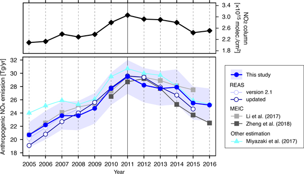
Table 1. Summary of NOx emission variations before and after 2011 over China.
| Period | ||||
|---|---|---|---|---|
| Study | Method | 2005−2011 | 2011−2015 | 2011−2016 |
| This study | Top-down | +1.4 (+5.6) | −0.8 (−2.9) | −0.8 (−3.0) |
| REAS updated | Bottom-up | +1.7 (+7.1) | −1.3 (−4.5) | − |
| Li et al (2017b) | Bottom-up | +1.3 (+5.4) | −0.5 (−1.8) | − |
| Zheng et al (2018) | Bottom-up | − | −1.4 (−5.2) | −1.4 (−5.4) |
| Miyazaki et al (2017) | Top-down | +1.0 (+3.9) | −1.1 (−4.0) | −1.2 (−4.1) |
Note. Units: Tg yr−1 (%/year).
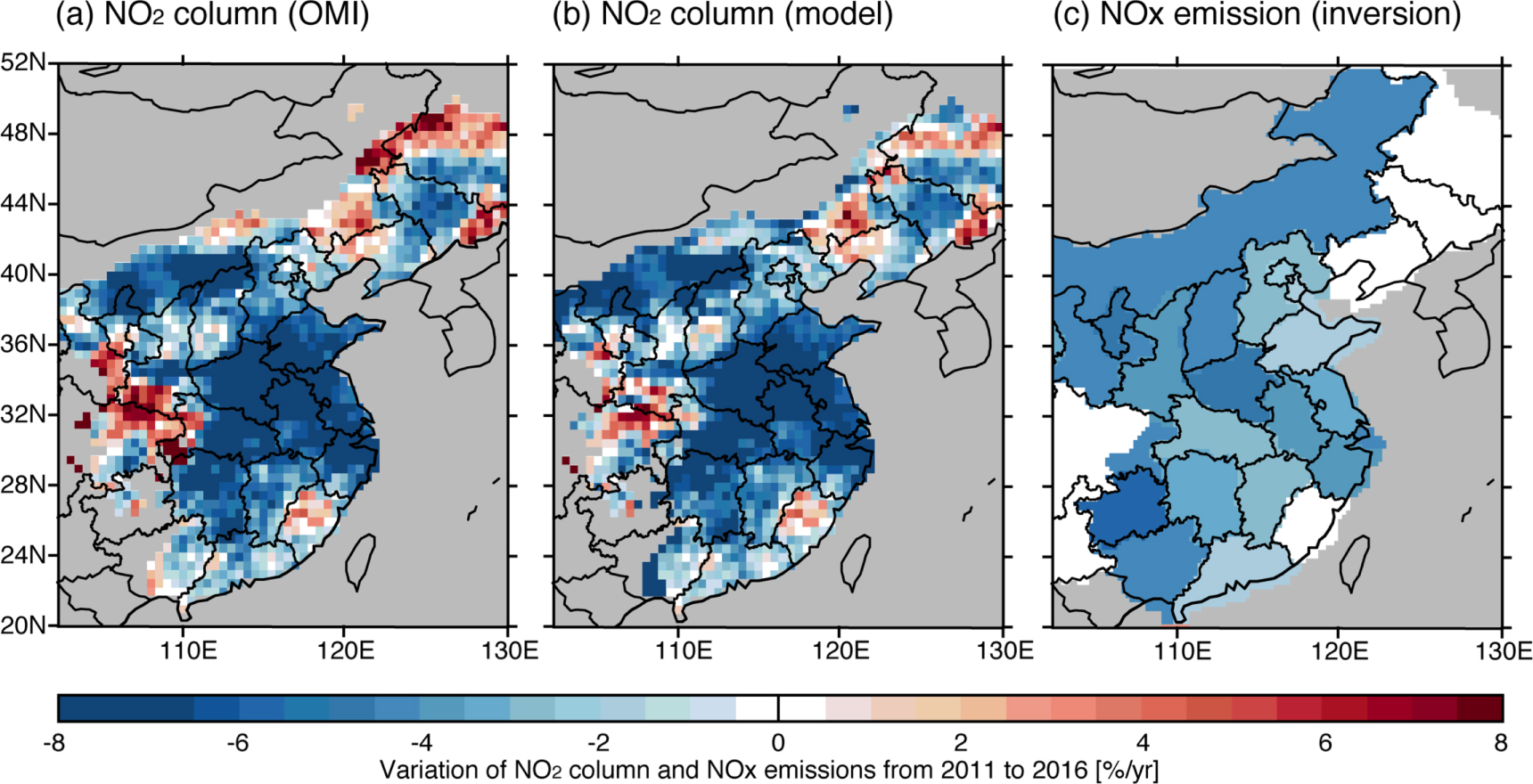
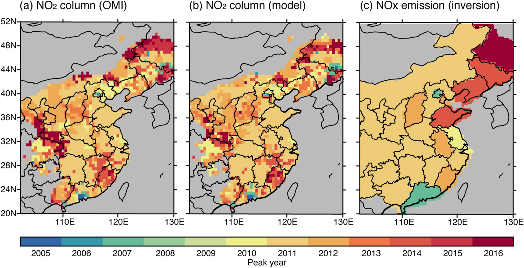
The variation over China is shown in figure 1, and we focused on eastern China, particularly over the centers of population and economic activity. Figure 2 shows the annual trends from 2011 to 2016. Generally, there were decreasing trends, although there were some increasing trends over parts of Sichuan Province, Fujian Province, and northeast China. The observed and modeled NO2 column showed similar variations and the trends with the largest changes of greater than −10%/year were centered on eastern China (i.e. Henan, Hubei, and Anhui Provinces). The inverse estimated emissions on the province scale showed trends of around −3%/year and there were large differences according to location. Our inverse estimate of NOx emissions from China as a whole showed the peak in 2011, whereas the estimation by Zheng et al (2018) showed the peak in 2012 (figure 1). Figure 3 shows the peak year of the observed and modeled NO2 column and inverse estimated NOx emissions on the province scale in China. The peak year of the observed and modeled NO2 column corresponded well; generally, the peak year was around 2011 (light orange), Beijing and Guangzhou exhibited an earlier peak between 2005 and 2008 (blue to green), and northeast China exhibited a later peak between 2013 and 2016 (red).
Figure 2. Variation of (a) NO2 column observed by OMI (Ωo), (b) modeled NO2 column (Ωa), and (c) inverse estimated NOx emissions on the Chinese province scale from 2011 to 2016.
Download figure:
Standard image High-resolution image
Figure 3. Spatial distribution of the peak year for (a) NO2 column observed by OMI (Ωo), (b) modeled NO2 column (Ωa), and (c) inverse estimated NOx emissions on the Chinese province scale.
Download figure:
Standard image High-resolution image
3.2. Continuous increase over India
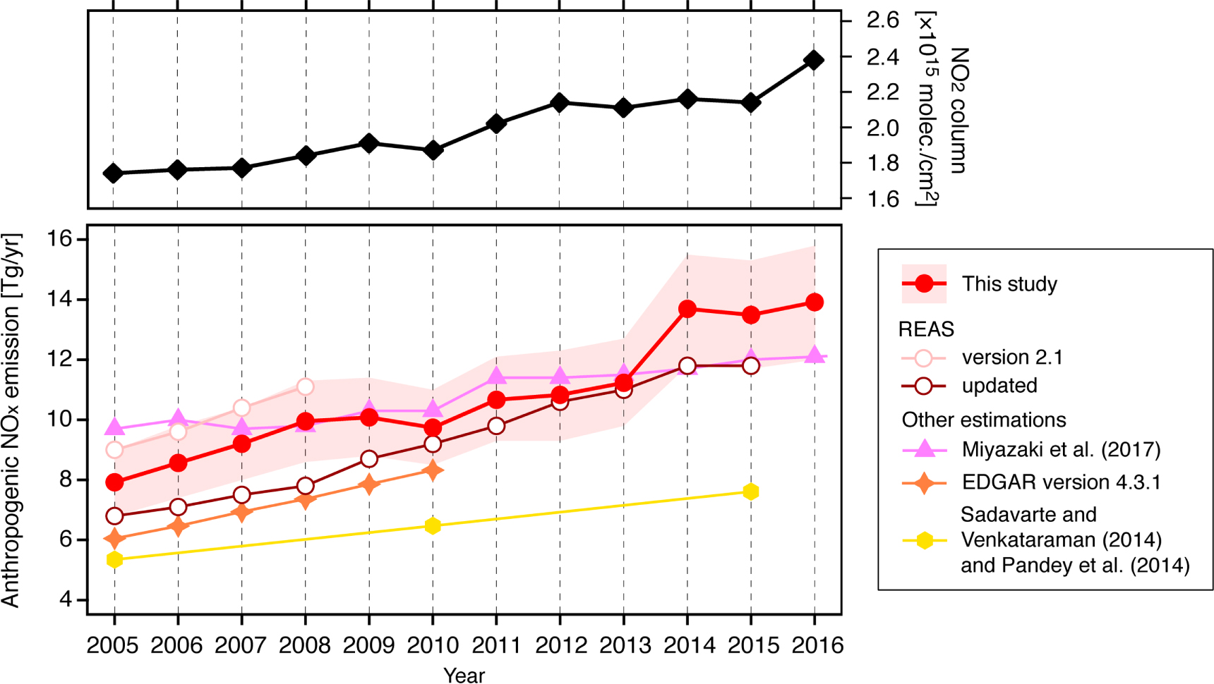
The observed NO2 column and estimated NOx emissions over India with estimated error are shown in figure 4. NOx emissions increased continuously over India from 2005 to 2016. In contrast to China, NOx emissions increased in most parts of India (results not shown). Other emissions taken from the updated REAS inventory (Kurokawa et al 2018), the inverse estimation by Miyazaki et al (2017), the Emission Database for Global Atmospheric Research (EDGAR) version 4.3.1 (http://edgar.jrc.ec.europa.eu/index.php), and the emissions dataset from a technology-linked inventory over India (Pandey et al 2014, Sadavarte and Venkataraman 2014) are also shown. The analyzed periods were 2005–2010, 2005–2015, and 2005–2016, and the variations in our estimation and other emission estimations are summarized in table 2. The changes were +0.1 to +0.6 Tg yr−1 (+1 to +6%/year) from 2005 to 2010 and +0.2 to +0.6 Tg yr−1 (+2 to +6%/year) from 2005 to 2015 or 2016. Our estimate shows a different trend from that in the observed NO2 column during 2014–2015. One possible reason for this is meteorological variability. The meteorological impacts on the relationship between NOx emission and tropospheric NO2 column amount should be analyzed in detail in future studies. In our estimation, there was a large increase during 2013–2014. The latest EDGAR for greenhouse gases emission inventory (https://edgar.jrc.ec.europa.eu/overview.php?v=CO2andGHG1970-2016) also report a similar large increase in CO2 emissions (ca. 10%/year) during 2013–2014, and this year-on-year growth rate is greater than in other years (ca. 5%–6%) between 2005 and 2016. Therefore, the increase in fossil fuel consumption could be one plausible reason for the large increase of our estimated NOx emissions during 2013–2014. Although there were differences in the rate of increase, all estimations indicated a continuous increase in emissions over India, in contrast to the varying trend over China.
Figure 4. Temporal variation of (top) annual NO2 column observed by OMI, and (bottom) annual NOx emission amounts over India during 2005–2016. REAS, EDGAR, and works by Sadavarte and Venkataraman (2014) and Pandey et al (2014) are bottom-up estimations, and Miyazaki et al (2017) used top-down estimations. The range of our estimations represents the error of the a posteriori emissions. Note that the error of the a priori emissions (REAS version 2.1) over India is ±49%.
Download figure:
Standard image High-resolution image
Table 2. Summary of NOx emission variations during 2005–2016 over India.
| Period | ||||
|---|---|---|---|---|
| Study | Method | 2005−2010 | 2005−2015 | 2005−2016 |
| This study | Top-down | +0.4 (+4.4) | +0.5 (+4.9) | +0.5 (+4.9) |
| REAS updated | Bottom-up | +0.5 (+6.2) | +0.6 (+6.0) | — |
| Miyazaki et al (2017) | Top-down | +0.1 (+1.1) | +0.3 (+2.4) | +0.2 (+2.3) |
| EDGAR version 4.3.1 | Bottom-up | +0.5 (+6.4) | — | — |
| Sadavarte and Venkataraman (2014) and Pandey et al (2014) | Bottom-up | +0.2 (+3.8) | +0.2 (+3.5) | — |
Note. Units: Tg yr−1 (%/year).
3.3. Future perspectives on emission variations over China and India
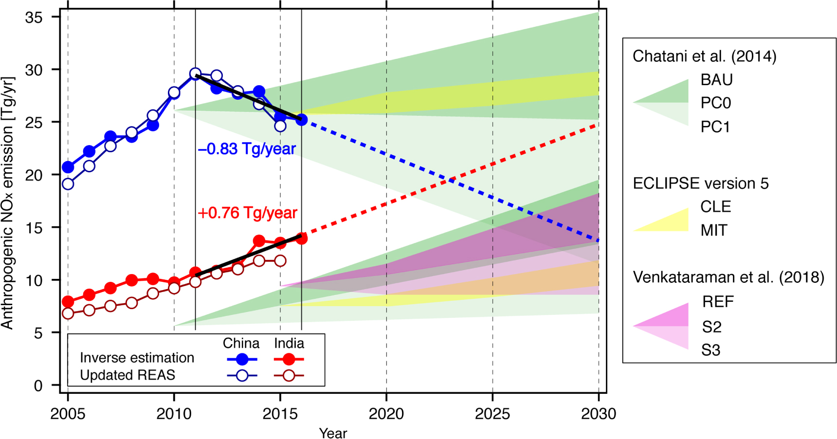
Our inverse NOx estimation over China and India showed a reversal in the increase in emissions after 2011 over China and a continuous increase over India. In this section, we provide perspectives for future emission changes in China and India. Based on the inverse estimation in this study, the NOx emission trend was −0.83 ± 0.14 Tg yr−1 over China and +0.76 ± 0.16 Tg yr−1 over India with a significance level of p < 0.005 (Students’ t-test) during 2011–2016 (figure 5). The peak year of NOx emission from China was set as 2011 in the trend analysis. Future scenarios reported in several other studies are also included in figure 5. Chatani et al (2014) (shown in green in figure 5) estimated three scenarios based on business as usual (BAU), additional legislation and technological developments (PC0), and legislation and developments beyond those in PC0 (PC1) over China and India in 2030 based on 2010 emissions. The European Union’s project of Evaluating the Climate and Air Quality Impacts of Short-Lived Pollutants (shown in yellow in figure 5; Stohl et al 2015) created current legislation (CLE) and short-lived climate pollutant mitigation (MIT) scenarios from 2015 to 2050 over China and India. Venkataraman et al (2018) (shown in red in figure 5) reported emission pathways based on reference (REF), aspirational (S2), and ambitious (S3) scenarios from 2015 to 2050 over India.
Figure 5. Future perspectives for NOx emission variation over China and India for scenarios reported in the literature and our inverse estimations.
Download figure:
Standard image High-resolution image
Over China, current reduction trends after 2011 are beyond the expected regulation. Both the PC0 and MIT scenarios foresaw almost flat trends for NOx emissions from China; however, all top-down and bottom-up estimates after 2011 suggested declining trends (figure 1 and table 1). The current decreasing trends are consistent with the projected regulation in the PC1 scenario with decreases of 0.7 Tg yr−1 (3.9%/year). In contrast, the increasing trends over India match the unregulated scenarios of 0.7 Tg yr−1 (5.5%/year) for BAU, 0.3 Tg yr−1 (2.9%/year) for CLE, and 0.6 Tg yr−1 (4.2%/year) for REF. Based on the confirmation of our recent estimation trends over China and India with various future scenarios, we assume continuous trends of −0.83 ± 0.14 Tg yr−1 over China and +0.76 ± 0.16 Tg yr−1 over India after 2016. Under this assumption, NOx emissions from China and India will be similar in 2023 with around 19–20 Tg yr−1, and NOx emissions from India will surpass those from China in 2024. Based on the range of the trends, the excess NOx emissions from India rather than China will occur between 2022 (maximum decrease of −0.97 Tg yr−1 over China and maximum increase of +0.92 Tg yr−1 over India) and 2025 (minimum decrease of −0.69 Tg yr−1 over China and minimum increase of +0.60 Tg yr−1 over India). Because the US, which is the second largest source, has shown a decline of −0.65 Tg yr−1 during 2011–2016 (https://epa.gov/air-emissions-inventories/air-pollutant-emissions-trends-data) or even in the possible slowdown trend (Jiang et al 2018), India will become the world’s largest NOx emission source. These are the first perspectives for future emission changes to two importance sources in Asia, and we should continue to monitor these changes closely.
4. Conclusion
We developed an immediate inversion system to estimate NOx emissions using the constraint of NO2 column density satellite observations. Our inversion system, which is based on the linear unbiased optimum estimation, improves upon previous studies because it can be used to update emissions quickly and simply, it considers errors for both the model and observations, and it includes model bias. In this study, we used our system for the inverse estimation of long-term variation of NOx emissions over China and India from 2005 to 2016. The results showed that NOx emissions from China peaked in 2011, and subsequently declined by around 1.0 Tg yr−1 (around 3%/year), consistent with other estimates. Compared with the large variation found over China, NOx emissions from India increased continuously by 0.1–0.6 Tg yr−1 (1 to 6%/year). Based on these contrasting trends over China and India, we predicted the following future trends in NOx emissions over Asia. Our inverse estimation indicated a decrease of 0.83 Tg yr−1 over China and an increase of 0.76 Tg yr−1 over India from 2011 to 2016, corresponding to strictly regulated and unregulated future scenarios, respectively, as reported in several studies. Assuming continuous trends after 2016, we expect that NOx emissions from India will surpass those from China in 2024, and India will become the largest global NOx emission source.
Acknowledgments
This work was partly supported by the Global Environment Research Fund (No. S-12, 5-1903) of the Ministry of the Environment, Japan. This work was also funded by a collaborative research program through the Research Institute for Applied Mechanics (RIAM) at Kyushu University (No. 30 AO-14, 2019 AO-11). This work was also supported by JSPS KAKENHI JP16H02946. Part of the research was carried out at the Jet Propulsion Laboratory, California Institute of Technology, under a contract with the National Aeronautics and Space Administration. The authors acknowledge T Noguchi for his technical support.
Data availability statement
The data that support the findings of this study are available from the corresponding author upon reasonable request.