SQL Window Functions: All You Need to Know About Using Them

SQL’s versatility as a DBMS querying language has risen over the years. Its expansive utility and versatility make it an all-time favorite for every data analyst.

There are quite a few advanced-level functions besides SQL’s regular ones. These functions are commonly known as window functions. If you’re dealing with complex data and want to perform advanced calculations, you can use them to make the best use of your data.

The Importance of Window Functions

Several window functions are available in SQL, and each will help you perform a series of calculations. From creating partitions to ranking rows or assigning row numbers, these window functions do a little bit of everything.

Window functions are beneficial when you’re applying aggregate functions over a specific dataset, or collection of rows. These functions go above and beyond the aggregation functions that GROUP BY provides. However, the main difference is that, unlike the grouping function, your data is not combined into a single row.

You can't use window functions within the WHERE, FROM, and GROUP BY statements.

Syntax of a Window Function

When you refer to any window function, you need to follow the default syntax structure, so that it functions correctly. If you structure the command incorrectly, you’ll get an error and your code will fail to run.

Here's the default syntax:

SELECT columnname1,
{window_function}(columnname2)
OVER([PARTITION BY columnname1] [ORDER BY columnname3]) AS new_column
FROM table_name;

Where:

• coulmnname1 is the first column name you would like to select.
• {window_function} is the name of an aggregate function like sum, avg, count, row_number, rank, or dense_rank.
• columnname2 is the name of the column on which you’re applying the window function.
• columnname3 is the third column name, which will form the base for partition.
• new_column is a label for the new column you can apply using the AS keyword.
• table_name is the name of the source table.

Window functions are different from some of the most basic SQL commands. Unlike aggregate functions in SQL, you can use these window functions to perform advanced functions.

Preparing the Dataset

You can use the CREATE TABLE statement to create a new table in SQL. Here's a sample dataset that this guide will use to define some window functions:

The Sum Function Explained

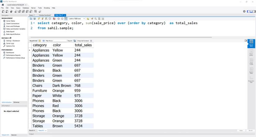
Suppose you want to calculate the total sales for each value within the category column. Here's how you can do it:

SELECT category, color,
sum(sale_price)
OVER (order by category) AS total_sales
FROM sahil.sample;

In the above code, the SQL statement pulls the category and color from the original dataset. The sum function adds up the sale_price column. It does so by category, since the OVER clause specifies ordering by the category column. The final result is as follows:

How to Use the Avg() Window Function

Like the sum function, you can calculate the average per row of data with the avg function. Instead of the sum, you will get a column with the average sales.

SELECT category, color,
avg(sale_price)
OVER (order by category) AS avg_sales
FROM sahil.sample;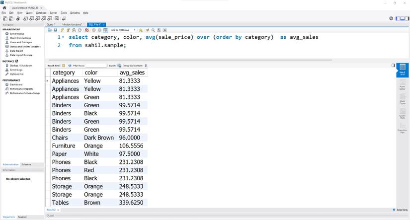

Learn to Use the Count() Window Function

Similar to the sum and avg functions, the count window function in SQL is pretty straightforward and works along the same lines as the other two functions. When you pass the count function, you get the total count of each value within the new column.

Here's how you can calculate the count:

SELECT category, color,
count(category)
OVER (order by category) AS item_count
FROM sahil.sample;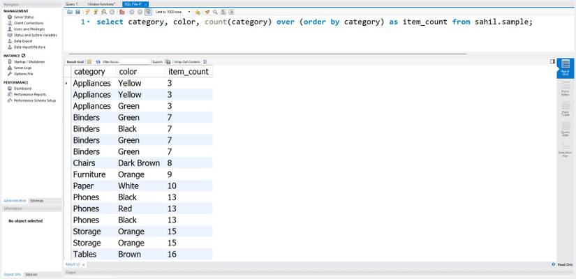

The Row_Number() Window Function

Unlike some of the other window functions listed above, the row_number() works slightly differently. The row_number() function assigns a row number to each row, depending on the order by clause. The starting row number is 1; the row_number assigns a corresponding value to each row until the end.

Here's the basic structure of a row_number() function:

SELECT category, color,
row_number()
OVER (order by category) AS item_number
FROM sahil.sample;

But what happens if you want to assign separate row numbers to each category item? The above syntax sets a rolling serial number, irrespective of the items stored within the category. For example, the appliances' category should have its exclusive numbering, followed by binders, and so forth.

You can use the partition function to perform this simple, yet practical task. The partition keyword assigns designated row numbers basis each category item.

SELECT category, color,
row_number()
OVER (partition by category order by category) AS item_number
FROM sahil.sample;

The Rank() and Dense_Rank() Functions

The rank() function works differently than the row_number() function. You need to specify the column name within the order by function, to use it as a base to define the rank values. For example, in the following code example, you can use the color column within the order by function. The query will then use that order to assign a rank value to each row.

You can use the code syntax below to pass a rank function in SQL:

SELECT category, color,
rank()
OVER (order by color) AS item_rank
FROM sahil.sample;

Take a look at the output to understand how this function works.

The order by function sorts the color category, while the rank function assigns a rank to each color. However, all the same color values have the same rank, while the different colors have separate ranks. The color black occurs thrice within the dataset; instead of assigning a rank value of 1, 2, and 3, the black color items get a rank of 1.

However, the next color Brown gets a rank 4 instead of rank 2. The rank function skips values and assigns the next chronological value to the different entries. If you want to assign a more meaningful rank value, you can use the dense_rank() function.

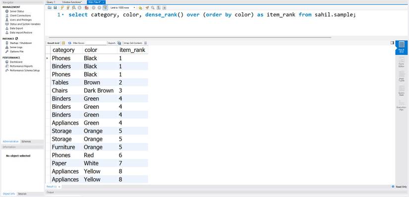
The dense_rank function doesn't skip any rank values during the order by function. For example, the first three color items (Black) will have rank 1. However, the following color (Brown) won't have a rank 4, but a rank 2, which is the following chronological number in the numbering list. The dense_rank function is a more practical window function as it assigns a meaningful value to the list of items.

Here's how you can use the dense_rank function in SQL:

SELECT category, color,
dense_rank()
OVER (order by color) AS item_rank
FROM sahil.sample;

And here’s an example of what the output from this function will look like:

SQL Functions to the Rescue

SQL’s window functions are ideal for carrying out advanced analytical operations. However, you can use plenty of other SQL commands to ensure your computational skills are top-notch. When you combine and calculate multiple results in one go, there is nothing better than using SQL's sub-queries.

Sub queries are an excellent tool to perform advanced functions, enhancing your results' quality. Depending on the need of the hour, you can customize your queries and make them more effective to suit your requirements.