1. Introduction
The flurry of activity, both observational and theoretical in nature, since the van Dokkum et al. (2015) study that coined the term ultradiffuse galaxies (UDGs) to describe physically large low-surface-brightness galaxies, has focused on understanding how these systems form and whether those processes highlight novel galaxy formation pathways or reflect extreme forms of already known phenomena. Challenges in resolving this question include: (1) a lack of homogeneous UDG data across environments; (2) the possibly heterogeneous nature of the objects selected using arbitrary physical size and surface brightness criteria (see Trujillo et al. 2020; Li et al. 2022, for attempts to define more physically motivated criteria); and (3) a paucity of constraints on the underlying dark matter halos that host these systems.
The first of these challenges we address with our search for UDGs in the images provided by the Dark Energy Spectroscopic Instrument (DESI) Legacy Imaging Surveys (hereafter referred to as the Legacy Survey; Dey et al. 2019). We have described the basic principles of our work with the survey data and provided candidate UDG catalogs across subsets of the data in three papers (Zaritsky et al. 2019, 2021, 2022, hereafter Papers I, II, and III, respectively). We refer to the survey as "SMUDGes," which stems from the survey’s full title, Systematically Measuring Ultra-Diffuse Galaxies. Here we present our complete catalog by augmenting a previous release of our analysis of the southern portion of the Legacy Survey (Paper III) with an analysis of the northern portion that we describe here in detail. Following most of the previous literature, we primarily identify candidates by applying a criterion based on central surface brightness in the g band, μ0 ≥ 24 mag arcsec−2. Specific to this survey, we also require candidates to have an angular half-light radius, re ≥ 5farcs3. This peculiar size limit was set to correspond to a physical re = 2.5 kpc at the distance of the Coma cluster, the environment explored by the first UDG surveys (Koda et al. 2015; van Dokkum et al. 2015; Yagi et al. 2016). Unfortunately, selecting on angular size but defining UDGs in terms of physical units exacerbates the problem that any sample of UDG candidates is a heterogeneous population of galaxies.
The heterogeneity of the UDG samples and the initial overestimated masses of some UDGs (see van Dokkum et al. 2016) has led to apparently conflicting results regarding the classification of UDGs. Studies of individual UDGs (e.g., Beasley et al. 2016; Toloba et al. 2018; van Dokkum et al. 2019b; Forbes et al. 2021), which naturally focus on the largest, brightest objects, tend to conclude that these are relatively massive galaxies (with total masses within the virial radius, including baryonic and dark matter, Mh , roughly comparable to, or larger than, that of the Large Magellanic Cloud, Mh ∼ 1.4 ×ばつ 1011 M⊙; Erkal et al. 2019), while studies using statistical samples of UDGs (e.g., Beasley & Trujillo2016; Amorisco et al. 2018), which naturally focus on the more numerous smaller objects, tend to conclude that UDGs are lower-mass galaxies (Mh < 1011 M⊙). However, the discrepancy is sometimes just a matter of emphasis. For example, the result of Sifón et al. (2018), who placed a statistical limit on UDG halo masses from gravitational lensing of log(M200/M⊙) ≤ 11.8 with high confidence, is sometimes cited as falling in the low-mass camp simply because it is compared to the initial claims that some UDGs could have Mh ≥ 1012 M⊙ (van Dokkum et al. 2016).
Reliable total mass measurements for statistical samples of UDGs are critical because we can use them to assess the degree to which these galaxies have underproduced stars, or "failed," during their existence. The first formation scenario for UDGs posited that the loss of gas at early times in dense environments led to massive failed galaxies in the Coma cluster (van Dokkum et al. 2015). This suggestion was quickly followed up by an opposing model where it was proposed that UDGs represent the tail of high-angular-momentum halos, interpreting UDGs instead as "puffy" low-mass galaxies (Amorisco & Loeb 2016). Subsequently, numerical simulations have introduced a number of other possible evolutionary factors (for some examples, see Di Cintio et al. 2017; Chan et al. 2018; Martin et al. 2019; Wright et al. 2021). Although the situation is clearly more complex than suggested by early toy models, empirical estimates of Mh are constraining for any scenario.
The other factor that is often cited as critical in UDG formation is the environment (e.g., Safarzadeh & Scannapieco2017; Chan et al. 2018; Carleton et al. 2019; Sales et al. 2020; Wright et al. 2021). Interactions, either with individual galaxies or with the global environment, are often invoked to truncate star formation and produce the typically quiescent appearance of UDGs (van Dokkum et al. 2015; Safarzadeh & Scannapieco 2017; Chan et al. 2018; Grishin et al. 2021). The identification of UDGs in the field (e.g., Martínez-Delgado et al. 2016; Román & Trujillo 2017; Leisman et al. 2017; Greco et al. 2018) directly demonstrates that dense environments are not necessary for UDG formation. However, even more restrictive are subsequent observations that appear to show little if any change in the number of UDGs per total host environment mass across a wide range of environments (van der Burg et al. 2016, 2017; Román & Trujillo 2017; Karunakaran & Zaritsky 2023; Goto et al. 2023). If environment plays a role beyond quenching star formation (UDG color does depend on environment; Prole et al. 2019; Kadowaki et al.2021), creation and destruction of UDGs must be delicately balanced.
Our challenge is therefore fourfold. First, identify a sample of UDG candidates across environments in sufficient numbers for statistical study. This we do as described in Papers I–III and complete that task here (Sections 2, 3, and 4). Second, estimate distances for as large a fraction of those candidates as possible to determine which candidates satisfy the UDG size criterion. We do this using the distance-by-association technique presented in Paper III (Section 4.1). As larger samples of spectroscopic redshifts become available, the method will become more robust, so although we present our distance estimates, we consider this to be a living catalog that will improve with time. Third, provide a measurement of the local environment (Section 4.2). Such an estimate is a byproduct of our distance estimation technique (Section 4.1). Finally, estimate Mh for as large a sample as possible, which we do in Section 4.3 using the technique presented by Zaritsky & Behroozi (2023). We close by discussing the implication of our mass measurements on the star formation efficiency of UDGs in Section 5. We use a WMAP9 ΛCDM flat cosmology throughout with Ω = 0.287, and H0 = 69.3 km s−1 Mpc−1 (Hinshaw et al. 2013). Magnitudes are on the AB system (Oke 1964; Oke & Gunn 1983).
2. The Data
We report the results of our analysis of Data Release 9 (DR9) of the northern portion of the Legacy Survey, which includes observations obtained by the MOSAIC camera at the KPNO 4 m telescope (MzLS, Mayall z-band Legacy Survey) and the 90Prime camera (Williams et al. 2004) at the Steward Observatory 2.3 m telescope (BASS, Beijing–Arizona Sky Survey). In addition to these telescopes, the full survey also employs DECam (DECaLS) at the CTIO 4 m, which was the focus of our previous work described in Papers I–III. This paper presents our final SMUDGes catalog release, and we do not intend to reprocess data using DR10 or any future release.
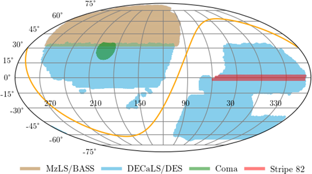
Briefly, the Legacy Survey (Dey et al. 2019) was initiated to provide targets for the DESI survey drawn from deep, three-band (g = 24.7, r = 23.9, and z = 23.0 AB mag, 5σ point-source limits) images. That survey covers about 14,000 deg2 of sky visible from the northern hemisphere between declinations approximately bounded by −18° and +84°. The footprint of DR9 (Figure 1) also includes an additional 6000 deg2 extending down to −68° imaged at the CTIO by the Dark Energy Survey (The Dark Energy Survey Collaboration 2005). As shown in the figure, the footprint of MzLS and BASS (hereafter, jointly referred to as MB) has three-band coverage of about 5000 deg2 at declinations ≳32° with about 300 deg2 overlapping the region observed by DECaLS.
Figure 1. Footprint of the sky covered in all three bands by the DR9 release of the Legacy Survey (Dey et al. 2019). Observations used in this study from the northern part of the Legacy Survey are shown in tan (MzLS and BASS, jointly referred to as MB). Footprints of our previous work in Coma (Paper I), Sloan Digital Sky Survey Stripe 82 (Paper II), and the full southern region of the Survey (DECaLS and DES; Paper III) are displayed in green, red, and blue, respectively. The Galactic plane is traced by the orange curve.
Download figure:
Standard image High-resolution image
Because of the significant differences between the instrumentation used for MB and DECaLS, we have modified the pipeline developed for DECam that was used in our earlier work. Although the basic approach remains similar, there are noteworthy changes at various steps that we describe below.
3. Processing MB
As previously mentioned, the northern Legacy Survey data comes from two different telescope/camera combinations. The MOSAIC camera (MzLS) provides imaging in the z band and consists of four 4096 ×ばつ 4096 CCDs with a scale of 0farcs26 pixel−1 and a field of view of ∼36′ (Dey et al. 2016; Schweiker 2016). Imaging in the g and r bands is obtained with the 90Prime camera (BASS), which contains four 4096 ×ばつ 4096 CCDs with a scale of 0farcs454 pixel−1 and a field of view of 1fdg08 ×ばつ 1fdg03 (Zou et al. 2017). BASS observations were taken from 2015 November 12 to 2019 March 7 and MzLS from 2015 November 19 to 2018 February 12. 7 As before, our processing and analysis of these data are performed on the Puma cluster at the University of Arizona High Performance Computing Center. 8
As in our previous work, we summarize the major steps in identifying potential UDGs as: (1) image processing that produces a preliminary list of candidates; (2) rejection of those that are likely to be Galactic cirrus contamination; (3) automated classification screening for false-positive detections; (4) visual confirmation of remaining candidates; (5) estimation of completeness, biases, and uncertainties using simulated sources; and (6) creation of the catalog. Details of these processes have been previously described and, other than brief summaries, we only address pipeline modifications here.
In a significant departure from our previous methodology, we now use the three-band coadded images generated by the Legacy Survey pipeline and publicly available on their website 9 in our UDG search. The Survey footprint is divided into 0.25 ×ばつ 0.25 deg2 "bricks" as described by Dey et al. (2019). During coaddition, the camera images are reprojected at a pixel scale of 0farcs262 with north up, converted into calibrated flux units of nanomaggies, and sky-subtracted. The actual brick sizes are 3600 ×ばつ 3600 pixel2, allowing a small amount of overlap. We limit our analyses to those included in the survey-bricks-dr9-north.fits.gz file, which is included in the Legacy Survey’s DR9. This file has information for each brick, including the median number of exposures in each filter. As in our earlier work, our automated classifier (Section 3.4) requires cutout images from all three bands and, therefore, we only include those bricks having at least one observation in each band. We further exclude a small number of observations (<1%) that were obtained in equatorial regions to cross-calibrate photometry with DECaLS and DES imaging (Dey et al. 2019), leaving 83,038 bricks for analysis of which about 6% overlap with DECaLS in the decl. range of ∼32°–34° (Figure 1).
3.1. Image Processing for MB
After downloading brick images and supporting files from the Legacy Survey website, we identify potential UDG candidates using the following steps:
- 1.Although the coadded images have already passed through the Legacy Survey pipeline, we additionally replace saturated pixels with values obtained from neighboring pixels using the methodology described in Paper I.
- 2.We remove objects on bricks that are clearly too bright to qualify as UDG candidates. As in Paper III, this is done using modeling to subtract sources that have SExtractor (Bertin & Arnouts 1996) MU_MAX values that are 2 mag arcsec−2 brighter than a specified threshold in each band (24.0 for g, 23.6 for r, and 23.0 for z).
- 3.A crucial step in our detection pipeline is the use of wavelet transforms with tailored filters to isolate candidates of different angular scales. When applied to all MB bricks, this results in a total of 46,374,815 detections, or an average of ∼558 per brick, the vast majority of which will not be classified as UDG candidates after further screening.
- 4.Spurious detections are limited by requiring that a potential candidate have coincident detections (defined as center-to-center separations <4′′), in at least two of the three bands, with the resulting group of detections considered to be located at the mean centroid position. This requirement rejects all but 7,238,447 wavelet detections and results in 3,521,143 separate groupings with an average of ∼42 groups per brick.
- 5.At this point in our pipeline, the vast majority of candidates will not survive further screening and, as described in our earlier work, we limit the number of detections requiring time-consuming GALFIT (Peng et al. 2002) modeling by obtaining much faster, rough parameter estimates using the LEASTSQ function from the Python SciPy library (Virtanen et al. 2020). Other than modeling detections on bricks rather than CCDs, our approach is unchanged from Paper III. Because this is only used as a coarse screen, we fit an exponential Sérsic model (n = 1) to each candidate on a brick and require that the results meet conservative parameter thresholds of re ≥ 4′′ and μ0 ≥ 23.0, 22.0 and 21.5 mag arcsec−2 for g, r, and z, respectively. In a departure from our previous work, we only require that a candidate successfully meet these criteria in one of the three bands comprising a brick, leaving a total of 624,469 detections comprising 499,866 distinct candidates that survive this step. Note that while changes such as this one will result in differences in the candidate UDGs between the southern and northern regions, some differences were unavoidable given the data quality differences. Nevertheless, we attempt to homogenize the catalog by evaluating measurement biases and completeness separately for the southern and northern surveys.
- 6.We perform an initial GALFIT screen of each candidate using a fixed Sérsic index of n = 1, without incorporating the point-spread function (PSF) into the model. In our prior work, we allowed GALFIT to generate its own sigma image, but we now provide one using the publicly available inverse variance images created by the Legacy Survey pipeline during coaddition. As in Paper III, we use generous acceptance thresholds of re ≥ 4′′, b/a ≥ 0.34, and μ0,g ≥ 23 mag arcsec−2 or μ0,z ≥ 22 mag arcsec−2 if there is no available measurement of μ0,g . A total of 86,746 candidates meet these criteria. Important details, such as masking, are described fully in Papers I, II, and III. Here we only note that the masking removes nearby objects, including any bright source at the center of the UDG candidate, to avoid the influence of possible nuclear star clusters in the model fitting. The central surface brightness that we use throughout our selection is that inferred from the fitted model, not one directly measured at the source center.
- 7.Our final image processing step uses GALFIT with a variable Sérsic index and an estimate of the PSF to model the remaining candidates as described in Paper III. We again use inverse variance images provided by the Legacy Survey to create the sigma image. In another departure from our earlier pipeline, we now use their PSF images to estimate the PSF by taking the median value of a 7 ×ばつ 7 pixel region centered on the candidate.
When we compare the initial results from our pipeline to matched DECaLS candidates in the overlapping region, we find large biases in the structural parameters and z-band photometry with much smaller differences for photometric estimates measured in the g and r bands. There are no significant biases when we reprocess these same candidates using bricks from DECaLS, indicating that the problem is not pipeline-related. Other than for re ≥ 10′′, where values using bricks are ∼25% less than those of CCDs, there are no significant biases in either structural or photometric estimates when we reprocess these same candidates using bricks from DECaLS. While some discrepancies, which seem to be limited to estimates of re at large effective radii, may be attributable to changes in the pipelines, the vast majority of the differences appear to be related to the processing of the MB images. Moreover, when we reprocess images from single filters using bricks, discrepancies for both re and photometric properties are isolated to the z-band and become more significant for the larger candidates. We attribute the behavior we find to oversubtraction of the background in DR9 processing of the z-band images of large, low surface brightness systems. 10 . The discrepancies in morphological parameters significantly improve when the z band is omitted from the stack. Therefore, we proceed without the z-band images in the stack. However, even with this modification, estimated effective radii are slightly smaller than those found in DECaLS. Fewer than 10% of our candidates have re ≥ 10′′, and we do correct for biases using our artificial source simulations, so we do not expect this modest discrepancy to affect our conclusions. This comparison highlights the problems inherent in comparing results from different telescopes using different pipelines; especially if there is no avenue for assessing relative biases.
After applying our final criteria of re ≥ 5farcs3, μ0,g ≥ 24 mag arcsec−2 (or μ0,z ≥ 23 mag arcsec−2 if GALFIT failed to model g), b/a ≥ 0.37, and n < 2, we are left with 22,866 candidates available for further evaluation.
3.2. Screening of Spurious Sources Caused by Cirrus
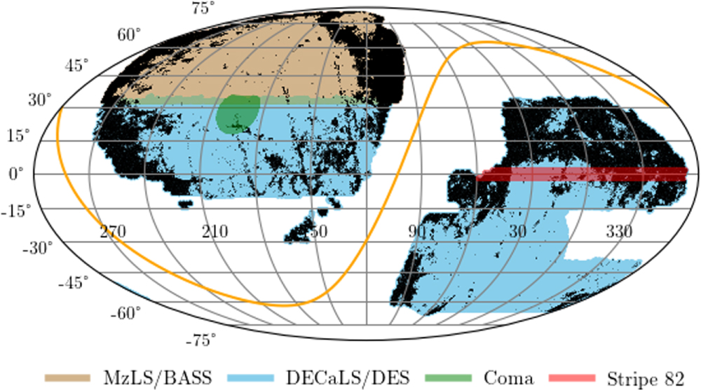
Large regions of the Legacy Survey footprint are contaminated by Galactic cirrus that can result in spurious detections that may be difficult to differentiate from legitimate UDG candidates (Figure 2). As in Paper III, we address this problem by rejecting as probable dust any candidates having single point values exceeding 0.05 in the τ353 dust map (Planck Collaboration et al. 2014) or 0.1 MJy sr−1 in the Wide-field Infrared Survey Explorer (WISE) 12 μm map (Meisner & Finkbeiner 2014). Using these criteria, we found in Paper III that 1.7% of the Coma region, ∼43% of the Stripe 82 footprint, and ∼31% of the entire DECaLS footprint exceeds these thresholds. As shown in Figure 2, about 22% of MB and 28% of the entire DR9 footprint are contaminated with cirrus. After applying the dust criteria to our candidates, a total of 14,388 are rejected, leaving 8478 in the MB footprint for further analyses.
Figure 2. Cirrus contamination within DR9 of the Legacy Survey footprint. Regions in black exceed our dust proxy thresholds of either 0.1 MJy sr−1 for WISE 12 μm map or 0.05 for τ353 and comprise ∼28% of the entire footprint. The Galactic plane is shown in orange.
Download figure:
Standard image High-resolution image
3.3. Screening of Duplicates
Before further processing, we eliminate duplicate entries, which we define as candidates lying within 10′′ of each other. We previously accepted the first entry of a group with duplicates and rejected the remainder. We now select the one with the smallest separation from the center of the cutout and reject the others on the assumption that the candidate with coordinates closest to those provided to GALFIT is the one most likely to be the desired entry. Because it is possible that detections separated by 10′′ could each represent a legitimate, distinct candidate, we visually inspected all 10 cases where separations were between 5′′ and 10′′ and found none that contained bona fide separate candidates. Most of the closely spaced duplicates result from detections of the same object in different bricks with one or more lying in an overlap region outside of the main 0.25 ×ばつ 0.25 deg2 brick area. Other causes include residual artifacts, tidal material, cirrus not rejected by our dust criteria, background clusters, and in a few cases, large, probably nearby, candidates that were detected multiple times during wavelet filtering. Our criterion eliminates 259 potential candidates, leaving 8219 for further classification.
3.4. Automated Classification
Our approach to computer classification is described in detail in the appendix of Paper I with modifications addressed in Paper II. Briefly, we use a convolutional neural network, which was trained on visually classified cutouts downloaded from the Legacy Survey in the Stripe 82 and Coma regions. We make no changes for the current study and use the prior trained network and weights for classification, resulting in 1415 of the 8219 being designated as UDG candidates. As explained in Paper II, based on visual inspection we find that objects with g − r colors >1.0 mag are unlikely to be UDGs and so reject 41 such objects from further consideration.
3.5. Visual Confirmation
As part of the development of our automated classifier in Paper II we found from visual examination that about 2.6% (8/306) of the candidates identified as potential UDGs in a test set were false positives. Paper III had similar results with about 2.8% (162/5760) being visually classified as false positives. We again wish to minimize the effects of false positives in our current catalog, and authors D.Z. and R.D. visually reviewed the 1374 remaining candidates in MB. Each reviewer initially classifies each candidate as a potential UDG, a false positive, or questionable. Those with disagreements or labeled as questionable are again classified by both reviewers. This procedure results in both reviewers labeling 1269 as UDG candidates and 80 as false positives with disagreement on 25. To minimize the number of false or ambiguous detections in our catalog, we consider any disagreements to be false positives resulting in 105/1374 (7.6%) being labeled as such. This fraction is almost triple those found in Papers II and III. We attribute this rise to our use of the training set drawn from stacked images obtained from DECaLS and DES, which are much deeper than the images used in the current study. 11 False positives are mitigated because all candidates are visually confirmed. A summary of all the screening steps is presented in Table 1.
To the extent that our simulations (Section 3.6) accurately represent actual UDGs, our estimates of completeness and bias should help compensate for differences in false negatives between the MB and DECaLS. Nonetheless, we attempt to quantify some of the causes of false negatives by investigating outcomes in the ∼300 deg2 region that overlaps both surveys at their abutting edges (Figure 1) with results shown in Figure 3. A total of 79 candidates from the northern and 88 from the southern contributions to this region made it through our entire pipeline, including visual confirmation. Of these, 64 were common to both surveys, leaving 15 (19%) in the northern portion and 24 (27%) in the southern portion unmatched.
Figure 3. Top panel: candidates found or missed in MzLS/BASS that are present in the DECaLS/DES catalog. Bottom panel: candidates found or missed in DECaLS/DES that are present in the MzLS/BASS catalog. Detection: inadequate or no wavelet detections (Section 3.1, Step 4); Sérsic: Failed to meet our Sérsic screening criteria (Section 3.1, Step 6); Galfit1: Failed our initial GALFIT screen (Section 3.1, Step 8); Galfit2: Failed our final GALFIT estimates (Section 3.1, Step 9); Classifier: Failed to meet the probability threshold required by our automated classifier (Section 3.4).
Download figure:
Standard image High-resolution image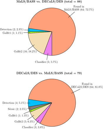
Only a few of the discrepancies resulted from undetected candidates and none because of visual confirmation. Most of the candidates not identified by the MzLS/BASS pipeline failed to meet our UDG criteria during final GALFIT modeling (Step 7 of Section 3.1). Although 13/16 had re ≥ 4′′, these did not meet our re = 5farcs3 threshold, and this was the most common cause of failure. This is not surprising since, as discussed (Section 3.1), GALFIT estimates of re for the northern survey tend to be smaller than those in the southern survey. Although our correction for this bias compensates for the difference in those surviving our entire pipeline, we still reject those that do not meet our UDG criteria at that point in the processing pipeline. About half of the candidates rejected by our automated classifier were close (>0.9) to the threshold (0.99) that we use for accepting a candidate (Paper II). Two candidates in DECaLS were rejected during Sérsic screening, likely because the individual CCD images processed in that study are noisier than the coadded bricks used in MzLS/BASS. This discussion highlights how sensitive membership is to the fine details of the data quality even when the analysis is done consistently, particularly near the limits of the selection criteria. We should not be surprised that a number of UDGs appear or disappear among different overlapping surveys because of different selection algorithms. We described similar results in Papers II and III, where we presented in more detail a comparison among catalogs from independent surveys. We recover most candidates in those surveys that satisfy the SMUDGes selection criteria. For example, when comparing to an H i-selected sample (Leisman et al. 2017), we recover 39 of 41 sources that match our selection criteria. Although in general we do find a few discrepancies, we conclude that there is no evidence for systematic biases among the surveys.
3.6. Estimating Completeness, Biases, and Uncertainties Using Simulated UDGs
In Papers II and III we estimated uncertainties and recovery completeness by planting simulated UDGs at random locations and separately processing them with the same pipeline as used for our real sources, including automated classification. Detailed descriptions and rationales for our approach to modeling are presented in Paper II with minor modifications and limitations discussed in Paper III and will not be repeated here except when needed for clarification. We continue to use Sérsic profiles with random structural and photometric properties, but because we now have a smaller footprint, we increase the initial simulation density from 600 to 1800 deg−2 (∼112 per brick). We further avoid brick overlap regions by restricting the central locations to only those pixels within the 0.25 ×ばつ 0.25 deg2 defined by the brick. Because we require a separation of at least 40′′ between simulations, the total number created is 7,295,356 for an average of about 88 per brick.
Our basic approach to modeling prevents us from including the full range of simulation parameter space. We mitigate the effects of this problem by expanding the thresholds used for our science candidates and accepting simulations with 22.5 < μ0,g < 27.5 mag arcsec−2, 3.5 < re < 20′′, b/a > 0.25, and 0.1 < n < 2 that also meet our dust and color criteria with 1,098,760 passing automated classification 12 .
As described in Paper II, all models use the four parameters that we consider the most appropriate for exploring the variable under consideration. Completeness and uncertainty estimates are obtained using polynomial models created with the PolynomialFeatures function from the Python Scikit-learn library (Pedregosa et al. 2011) and a four-layer neural network implemented with Keras. 13
3.6.1. Uncertainties
Parameter uncertainties for simulated sources are defined as the difference between final GALFIT values and the values used when creating the associated simulations (GALFIT − input). Because uncertainties are generally asymmetric, we define the bias as the median difference and the "1σ" confidence limits as the 15.1th and 84.9th percentiles of the distribution for a set of similar simulated objects.
Because polynomial models, especially of high order, may extrapolate very poorly for data points lying outside of the fitted range, our simulation range for individual parameters extends beyond those expected for our science targets. As in Paper III, we further mitigate this problem by using second-degree polynomial models to fit the simulation data. We continue to set all position angle, θ, biases to zero in the catalog because these values are negligible and we want to avoid adding noise.
3.6.2. Completeness
We define completeness as the probability that a candidate with given structural and photometric parameters will survive our entire pipeline. This is assessed using four modeled parameters (μ0,g , re , b/a, and n) and again uses a second-degree polynomial to fit the simulation results. We apply bias corrections to our catalog entries before estimating their completeness probabilities. Completeness for very large candidates, primarily in Virgo, was a problem in Paper III because our model re only extend to 20′′; however, no true candidate in the current study reaches that threshold, so this issue is not a concern here.
Table 1. Number of Detections and UDG Candidates in MB vs. Processing Step
| Process | Description in Text | Detections | UDG Candidates |
|---|---|---|---|
| Wavelet screening | Section 3.1, Step 3 | 46,374,815 | N/A |
| Object matching | Section 3.1, Step 4 | 7,238,447 | 3,521,143 |
| Sérsic screening | Section 3.1, Step 5 | 624,469 | 499,866 |
| Initial GALFIT screening | Section 3.1, Step 6 | N/A | 86,746 |
| Final GALFIT screening | Section 3.1, Step 7 | N/A | 22,866 |
| Cirrus screening | Section 3.2 | N/A | 8478 |
| Duplicate removal | Section 3.3 | N/A | 8219 |
| Automated classification | Section 3.4 | N/A | 1415 |
| Color criterion | Section 3.4 | N/A | 1374 |
| Visual Examination | Section 3.5 | N/A | 1269 |
Download table as: ASCII Typeset image
4. The Catalog
As noted in Section 3.5, there are 64 candidates common to DECaLS and MB. We omit these from the MB sample to avoid duplicate entries in the final merged catalog, leaving a total of 1310 new entries. Because we want to keep our simulation pipeline, which did not include visual examination, identical to our science pipeline, we retain in the catalog, but flag, candidates that we visually identified as false positives. These should be omitted from any conclusions drawn from our results. Descriptions of the catalog entries are presented in Table 2, and the full catalog is available. Each parameter entry includes its GALFIT estimate as well as its bias and confidence limits produced by our models. Any entry that required extrapolation of the fitted model beyond the range of the constraints is flagged and should be used with caution (Section 3.6). Users should apply the bias values by subtracting those presented in the catalog from the corresponding uncorrected measurements when drawing conclusions from the data.
Table 2. The Complete Catalog
| Column Name | Description | Format |
|---|---|---|
| SMDG | object name | SMDG designator plus coordinates |
| RA | R.A. (J2000.0) | decimal degrees |
| Dec | decl. (J2000.0) | decimal degrees |
| r_e | effective radius | angular (arcseconds) |
| r_e_upper_uncertainty | effective radius 1σ upper uncertainty | angular (arcseconds) |
| r_e_bias | effective radius measurement bias | angular (arcseconds) |
| r_e_lower_uncertainty | effective radius 1σ lower uncertainty | angular (arcseconds) |
| r_e_flag | effective radius uncertainty model flag | 0 = good, 1 = extrapolated |
| AR | axis ratio (b/a) | unitless |
| AR_upper_uncertainty | axis ratio 1σ upper uncertainty | unitless |
| AR_bias | axis ratio measurement bias | unitless |
| AR_lower_uncertainty | axis ratio 1σ lower uncertainty | unitless |
| AR_flag | axis ratio uncertainty model flag | 0 = good, 1 = extrapolated |
| n | Sérsic index | unitless |
| n_upper_uncertainty | Sérsic index 1σ upper uncertainty | unitless |
| n_bias | Sérsic index measurement bias | unitless |
| n_lower_uncertainty | Sérsic index 1σ lower uncertainty | unitless |
| n_flag | Sérsic index uncertainty model flag | 0 = good, 1 = extrapolated |
| PA | major axis position angle | defined to be [−90,90) measured |
| N to E, in degrees | ||
| PA_upper_uncertainty | major axis position angle 1σ upper uncertainty | degrees |
| PA_bias | major axis position angle measurement bias | degrees |
| PA_lower_uncertainty | major axis position angle 1σ lower uncertainty | degrees |
| PA_flag | major axis position angle uncertainty model flag | 0 = good, 1 = extrapolated |
| mu0_X | central surface brightness in band X (X ≡ g,r,z) | AB mag arcsec2 |
| mu0_X_upper_uncertainty | central surface brightness 1σ upper uncertainty in band X | AB mag arcsec2 |
| mu0_X_bias | central surface brightness measurement bias in band X | AB mag arcsec2 |
| mu0_X_lower_uncertainty | central surface brightness 1σ lower uncertainty in band X | AB mag arcsec2 |
| mu0_X_flag | central surface brightness uncertainty model flag in band X | 0 = good, 1 = extrapolated |
| mag_X | total apparent magnitude in band X | AB mag |
| mag_X_upper_uncertainty | total apparent magnitude 1σ upper uncertainty in band X | AB mag |
| mag_X_bias | total apparent magnitude measurement bias in band X | AB mag |
| mag_X_lower_uncertainty | total apparent magnitude 1σ lower uncertainty in band X | AB mag |
| mag_X_flag | total apparent magnitude uncertainty model flag in band X | 0 = good, 1 = extrapolated |
| Rejected | rejected based on visual inspection | 0 = good, 1 = rejected, |
| 2 = observers disagreed | ||
| SFD | optical depth at SMDG location from Schlegel et al. (1998) | unitless |
| A_X | corresponding extinction at SMDG location in band X | AB mag |
| Comp | fractional completeness for similar UDGs | unitless |
| Comp_flag | completeness model flag | 0 = good, 1 = extrapolated, |
| 2 = biases extrapolated | ||
| cz | recessional velocity | km s−1 |
| cz_type | redshift source | line-of-sight overdensity (OverDen), |
| cluster member (specific cluster name), | ||
| spectroscopic (specz) | ||
| sigma_est | estimated internal velocity dispersion | km s−1 |
| mass_h_est | estimate of log(Mh ) | log(M/M⊙) |
| env_sigma | σv of environment | km s−1 |
| env_n | number of galaxies in environment | |
| source | DECaLS (D) or MzLS/BASS (MB) |
Only a portion of this table is shown here to demonstrate its form and content. A machine-readable version of the full table is available.
Download table as: Data Typeset image
As mentioned in Section 3.1, because of systematic problems in the northern z-band stacked images, the magnitudes in MB tend to be higher than those in DECaLS. This offset is 0.5 mag and essentially independent of the estimated magnitude. Entries in the catalog are corrected for this bias by subtracting 0.5 mag from the GALFIT estimates for magz , and μ0,z is recalculated from these new values and the structural parameters assuming a Sérsic profile. Uncertainties and completeness are estimated from these revised entries. Nonetheless, all z-band entries for MB sources should be considered suspect and while they may be adequate for statistical conclusions, individual entries should be used with caution.
Parameters are corrected for bias before their completeness values are estimated. Completeness estimates may be suspect (Comp_flag ≠ 0) for either of two reasons. The parameters may be outside of the parameter space defined by our completeness model, and these have flag = 1. Alternatively, the bias correction derived from the uncertainty model may be unreliable, and these have flag = 2. In either case, the results should be used with caution.
Photometric parameters are not corrected for extinction, but extinction values are included in the catalog for those wishing to use them. Our extinction estimates (Ag , Ar , Az ) are calculated using the Sloan Digital Sky Survey g, r, and z Legacy Survey extinction coefficients 14 with E(B – V)SFD estimated using the dustmaps.py (Green 2018) SFD dust map based on the work of Schlegel et al. (1998).
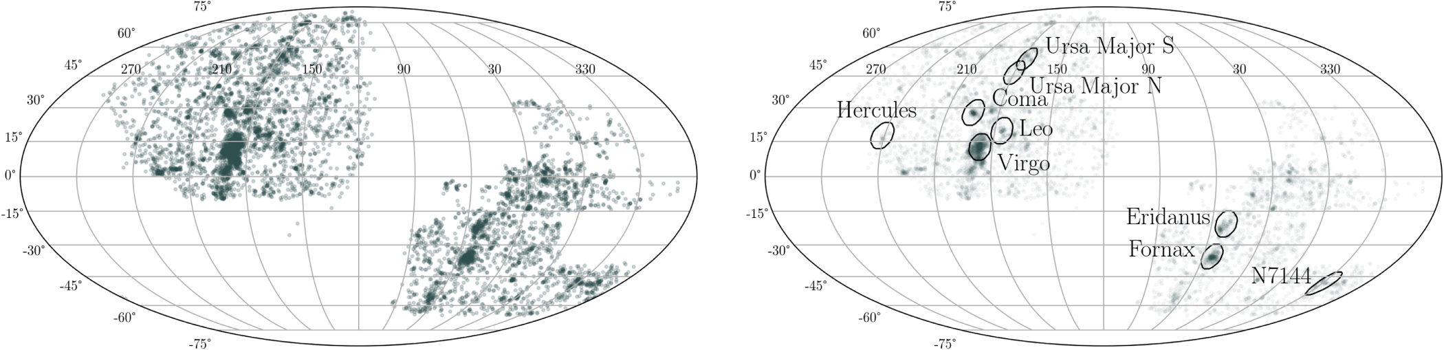
We recommend that images be reviewed in any study drawing conclusions based on individual candidates, particularly if those are extreme in any way (e.g., largest, faintest, etc.). The sky distribution of the merged SMUDGes catalog is shown in Figure 4. From now on, we discuss the merged southern and northern candidate sample.
Figure 4. The distribution of candidate UDGs across the sky in R.A. and decl. The right panel is the same as the left except that we have decreased the opacity of each point to help highlight the higher density regions. We label some well-known local overdensities for reference.
Download figure:
Standard image High-resolution image
4.1. Estimating Distances
Because UDGs are defined in terms of physical size, distance estimates are essential. This presents a challenge for our sample because it is not exclusive to rich galaxy clusters and groups. To estimate distances, we apply the distance estimation technique based on line-of-sight overdensities presented in Paper III. Additionally, we also assign those candidates projected onto the Coma, Fornax, and Virgo clusters, the richest clusters in our survey (Figure 4), the corresponding distance of the associated cluster. To reprise the former, we examine the distribution of galaxies with known redshifts around the line of sight to each UDG candidate, searching for possible overdensities with which to associate the candidate. We only include galaxies that are projected within 1.5 Mpc of the UDG candidate as calculated using the redshift of the galaxy in question. We assess whether the association with an overdensity is unambiguous using both a set of fixed criteria and machine learning. These criteria are described in detail in Paper III and result in the exclusion of any line of sight with multiple, independent overdensities that create ambiguity in the assigned redshift. We exclude objects with estimated cz < 1800 km s−1 so that we can reliably estimate the distance using its Hubble velocity. In Paper III we demonstrated that the technique has an accuracy rate of roughly 70% where accuracy is defined to mean that Δz < 3σz (σz is our estimate of the redshift uncertainty and corresponds to the velocity width of the associated line-of-sight galaxy grouping).
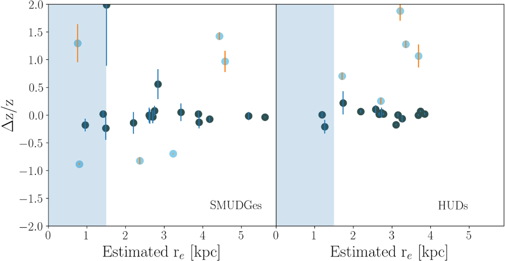
Using the complete catalog now available, and a few more UDGs with spectroscopic redshifts, we confirm (Figure 5) that this technique results in an accuracy of ∼70% when examining the SMUDGes candidates with measured redshifts (Kadowaki et al. 2021). The accuracy is 74% when examining the sample of H i-selected low surface brightness galaxies from Leisman et al. (2017). The results obtained for the latter sample show that the estimated redshift accuracy does not change appreciably when considering H i-rich galaxies, which presumably lie in lower-density regions. However, in either case, the redshift estimate yield is < 20% (18 and 13%, respectively), suggesting that we will only be able to estimate redshifts for a small fraction of the SMUDGes catalog using this technique and that the resulting sample may be skewed somewhat to denser-than-average environments.
Figure 5. Fractional redshift error vs. physical size. We plot the difference between the estimated and spectroscopically measured redshifts, divided by the redshift, as a function of inferred candidate size. The darker points represent candidates for which the estimate was within 3σ of the measured value, while those in the lighter symbols represent those for which it was not. The left panel contains results for SMUDGes candidates with spectroscopic redshifts from the Kadowaki et al. (2021) compilation and the right panel for Hi-selected ultradiffuse galaxies (HUDs) from Leisman et al. (2017). The shaded area highlights the region where the candidates are no longer classified as UDGs due to their small physical size.
Download figure:
Standard image High-resolution image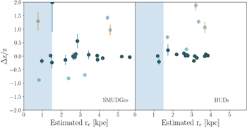
To complement this set of estimated redshifts, we assign any candidate without an estimated redshift and projected within 1, 1.5, and 2.3 Mpc from the Fornax, Virgo, and Coma clusters, respectively, the redshift of the host cluster. Finally, we include those candidates with spectroscopic redshifts (replacing any estimated redshift with the spectroscopic one).
In total, we present redshift estimates for 1525 candidates in the catalog and confirm as UDGs (re ≥ 1.5 kpc) 585 candidates. This UDG fraction is not expected to be representative for the survey because candidates in Virgo and Fornax, which are numerous and nearby, are far less likely to satisfy the physical re criterion given our angular size selection. The properties of these systems are presented in Figure 6. For the bulk of our candidates, we are unable to recover an estimated cz and validate them as UDGs. A priority for future research in this area must be expanding the reach of redshift estimation techniques. Nevertheless, there are alternative approaches, such as correlation analyses, that can bring the power of the full catalog to bear on certain questions (Prole et al. 2019; Greene et al. 2022; Goto et al. 2023). For the remainder of our discussion, we limit ourselves to the SMUDGes candidates with redshift estimates. Our estimates for the recessional velocities, czest, are included in the catalog, but they are likely to change in the future as the training sample and methodology improve.
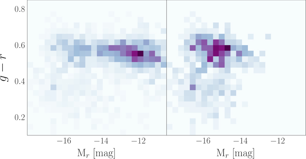
Figure 6. Color–magnitude distribution for SMUDGes candidates with estimated redshifts. In the left panel, we include all candidates with czest and in the right panel only those that at the estimated distance have re ≥ 1.5 kpc. The intensity scaling of each bin corresponds to a linear scaling of the number of objects in the bin, with different normalization in the two panels.
Download figure:
Standard image High-resolution image
As with the full catalog itself, we caution that in selecting samples of unusual objects, the likelihood of catastrophic failure becomes greater. For example, when selecting large (re ≥ 4 kpc), blue galaxies, the czest failure rate is closer to 50% (Table 3). The increase in the failure rate arises because blue galaxies are less likely to be physically associated with clear galaxy overdensities, and selecting the largest UDGs, which are rare, is likely to select for candidates with grossly overestimated values of czest . This overestimation is in fact the case for the three catastrophic failures (SMDG0031454+024256, SMDG0200102+284950, and SMDG0806124+153015).
Table 3. Redshift Comparison for Large Blue UDGs
| Name | Spectroscopic cz | Estimated cz |
|---|---|---|
| (km s−1) | (km s−1) | |
| SMDG0031454+024256 | 2377 | 4683 |
| SMDG0200102+284950 | 168 | 4874 |
| SMDG0803340+090730 | 4412 | 4619 |
| SMDG0806124+153015 | 1979 | 4803 |
| SMDG0915558+295527 | 7234 | 6711 |
| SMDG1601538+162909 | 10,626 | 10,464 |
Download table as: ASCII Typeset image
4.2. Estimating Environment
As a byproduct of the distance estimation technique, we have measurements of both the velocity dispersion of the associated overdensity and the number of galaxies in the overdensity. Both of these measurements have significant potential problems. We derive the velocity dispersion from the small number of galaxies in the associated group, and it has had the wings of the distribution trimmed (see Section 5 in Paper III). The number of galaxies in the overdensity is a strong function of the depth and completeness of the spectroscopic coverage, which varies across the sky. Nevertheless, it is reassuring that in a gross sense the two measurements track each other (Figure 7).
Figure 7. Comparison of two environmental tracers. The velocity dispersion, σv , and number of galaxies refers to the parameters of the overdensity associated with an individual UDG candidate. We show the results for all lines of sight, regardless of whether we accepted the estimated redshift. The two quantities track each other as expected, although with large scatter. Because of the large scatter, we choose to define the low-density environment as satisfying both σv ≤ 500 km s−1 and N < 15, and the high-density environment as satisfying both σv > 500 km s−1 and N ≥ 15. The selected regions are shaded and labeled.
Download figure:
Standard image High-resolution image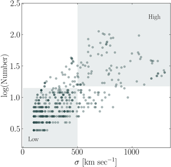
We use these two measures in concert to provide a broad guideline regarding the local environment of each UDG candidate for which a distance is estimated using this technique. Because of the significant scatter present in Figure 7, we opt to set joint limits and limit our environmental designation to solely rich (σv > 500 km s−1 and N ≥ 15) or poor (σv ≤ 500 km s−1 and N < 15) environments.
4.3. Estimating Masses
We follow the procedure described by Zaritsky & Behroozi (2023) and applied by Zaritsky (2022) to estimate total masses for as many of our UDG candidates with estimated distances as possible. The procedure divides into two steps.
First, we use a galaxy scaling relation to estimate the velocity dispersion of each galaxy. The scaling relation connecting re , the surface brightness within re , Ie , and velocity dispersion, σv across all types of stellar systems has been discussed extensively in a set of papers (Zaritsky et al. 2006, 2008). Having all but one of these parameters, the last can be estimated using the relation.
Second, we use the velocity dispersion to estimate the mass within re , subtract the contribution of baryons within re , and find the Navarro–Frenk–White (NFW; Navarro et al. 1997) model that has the corresponding dark matter mass within re . This estimate we test using globular cluster abundances for six UDGs. Both of these steps are described in more detail next.
4.3.1. Velocity Dispersion
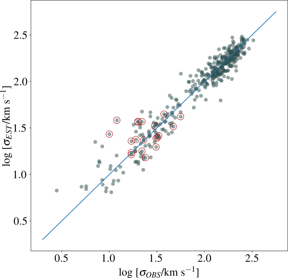
In Figure 8 we compare our estimated velocity dispersions, σEST, against spectroscopically measured values for a wide range of galaxies from the literature (references in Figure caption), and highlight UDGs (also drawn from published data). We use the empirically determined coefficients for the scaling relation given in Zaritsky & Behroozi (2023). With larger spectroscopic data sets, these coefficients should be further refined, particularly to better constrain the relationship in the region of parameter space populated by UDGs.
Figure 8. Comparison of estimated velocity dispersions of dispersion supported galaxies of various masses to the spectroscopically measured values (Jorgensen et al. 1996; Geha et al. 2003; Chilingarian et al. 2008; Mieske et al. 2008; Collins et al. 2014). Twenty UDGs with velocity dispersion measurements from the literature (Beasley et al. 2016; van Dokkum et al. 2017; Toloba et al. 2018; Chilingarian et al. 2019; Martín-Navarro et al. 2019; van Dokkum et al. 2019b; Forbes et al. 2021; Gannon et al. 2022) are highlighted with larger, open red circles. The dispersion about the 1:1 line for UDGs corresponds to a velocity dispersion scatter of 11 km s−1.
Download figure:
Standard image High-resolution image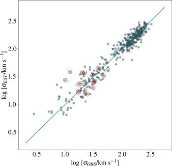
The UDGs follow the general trend on the 1:1 line and do not exhibit larger scatter than other galaxies of similar velocity dispersion. The rms scatter for the UDGs corresponds to 11 km s−1, roughly a $\sqrt{2}$ increase over the typical quoted uncertainty in the spectroscopic measurements, suggesting the estimated values have comparable precision to the spectroscopic ones. We propose that 11 km s−1 is a rough upper limit on the 1σ uncertainty of our velocity dispersion estimates. Of course, estimates have the potential for catastrophic errors and should always be treated with caution. We will return to this issue later, but the two UDGs with the lowest observed velocity dispersions suggest that the empirical relationship may be breaking down for low-velocity dispersion UDGs. We proceed to calculate σEST for every UDG candidate in the catalog with an estimated redshift. These estimates are included in the catalog but should be treated with caution and await further confirmation.
4.3.2. Modeling Total Masses
We estimate total masses by adopting an underlying NFW potential, determining the total mass within re using the Wolf mass estimator (Wolf et al. 2010), subtracting the stellar mass using a color dependent stellar mass-to-light ratio (Roediger & Courteau 2015) within re 15 , and finding the NFW profile that best matches the residual mass within re . This approach assumes that all of the baryons within re are in stars and that there is no adiabatic contraction of the halo due to the baryons. To help satisfy the latter assumption, we apply the method only to systems where the dark matter mass fraction within re is at least 50%. This effectively limits the technique to dwarf galaxies. Nevertheless, even if the original underlying potential was NFW-like, baryonic effects other than contraction, such as feedback, could also affect the shape of the potential (Sawala et al. 2013). Even so, there is yet no compelling argument that NFW potentials are inappropriate for UDGs (Sales et al. 2020), but whether this is an accurate assumption remains an open question.
There are limited ways to test the results of the method, including the assumption of the NFW profile, in galaxies in general—and even fewer in UDGs. We will use the relationship between the number of globular clusters, NGC, (or the total mass of the globular cluster population, which for a universal luminosity function is directly related to the number) and total galaxy mass, Mh , that is now well established for the general galaxy population (Blakeslee et al. 1997; Spitler & Forbes2009; Georgiev et al. 2010; Harris et al. 2013, 2017; Hudson et al. 2014; Forbes et al. 2016, 2018; Burkert & Forbes 2020; Zaritsky 2022). The relationship has already been assumed to hold for UDGs and used to estimate the total mass of many individual UDGs (e.g., Beasley & Trujillo 2016; Peng & Lim 2016; Amorisco et al. 2018).
In Figure 9 we compare NGC for a sample of six well-characterized UDGs (Saifollahi et al. 2022) and our estimates of Mh . The line plotted in the Figure is the relation obtained from the general galaxy population, Mh = (5 ×ばつ 109 M⊙)NGC (Burkert & Forbes 2020). If the published relation is taken as being correct, then our Mh estimates are underestimates of the total mass by ∼15% on average and have a scatter of ∼25%. If this evaluation of the accuracy and precision of the method is even close to being correct, it suggests that the method provides an exciting way forward to estimate masses for large numbers of low-mass galaxies, including UDGs. We present in the catalog our estimates for Mh for the subset of 1436 UDG candidates where we can proceed with the calculation.
Figure 9. The relationship between the number of globular clusters and total mass. The number of globular clusters comes from Saifollahi et al. (2022) and the masses come from our estimates. The dashed line is not a fit but rather the published relation from Burkert & Forbes (2020). The comparison indicates a modest offset and acceptable precision for our estimated masses (mean offset from the relation is 15%, and the scatter corresponds to an uncertainty in the mass of 25%). However, as detailed in the text, some exceptions to this behavior are known from other studies.
Download figure:
Standard image High-resolution image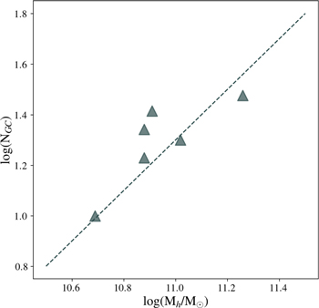
We chose to focus the NGC–Mh comparison on the Saifollahi et al. (2022) sample because NGC is based on deep HST imaging and a uniform treatment of selection and completeness corrections across the sample. However, a similar comparison has catastrophic failures when one considers a broader set of measurements. First, the two UDGs associated with NGC 1052 that have little or no apparent dark matter within re (van Dokkum et al. 2018a, 2019a) are clear outliers in this relation, independent of the mass estimation approach (van Dokkum et al. 2018b). They have substantial globular cluster populations but a low total mass. Although a variety of formation scenarios have been proposed for these systems, some are sufficiently fine-tuned (e.g., van Dokkum et al. 2022) to suggest that such objects should be exceedingly rare across the entire SMUDGes sample.
Also concerning is the case of NGC 5846 UDG1 (Forbes et al. 2019), although any one object may not be representative. Based on ground-based imaging, the galaxy appears to have a bountiful GC population (17 clusters initially identified, completeness corrections would more than double that number; Forbes et al. 2021), with 11 now spectroscopically confirmed (Müller et al. 2020). Using the scaling relation and the structural parameters presented by Forbes et al. (2019), we obtain σEST = 23 km s−1, in agreement with the published spectroscopic measurement, σv = 17 ± 2 km s−1 (Forbes et al. 2021). However, our subsequent estimate of the total mass is only 1.7 ×ばつ 1010 M⊙ in comparison to their estimate, based on NGC, of ∼2 ×ばつ 1011 M⊙. This is a factor of 10 discrepant, suggesting NGC would need to be ∼10 times smaller for us to place the galaxy on the relationship in Figure 9. There seems to be little room for observational error at this level. Subsequent HST observations (Müller et al. 2021; Danieli et al. 2022) confirm the large number of globular clusters, and adopting a subsequent measurement of σv using globular clusters (${\sigma }_{v}={9.4}_{-5.4}^{+7.0}$ km s−1; Müller et al. 2020) would make the discrepancy even worse because it lowers the inferred dynamical mass.
An alternative interpretation was suggested by Forbes et al. (2021) because they too found a conflict between the mass within re and the total mass. They suggest that the dark matter potential may be cored. If this is true, we would be underestimating the total mass by fitting an NFW model. Determining whether such discrepancies are common or isolated may be a way to learn about the dark matter potentials of these systems. We cannot make further progress here, but more careful study of the population of GC-rich low surface brightness galaxies is essential.
5. Star Formation Efficiencies
We now address whether the integrated star formation efficiency of UDGs is different than that of galaxies of similar total masses. We move forward with some trepidation given the chain of steps required to estimate masses, but are hopeful that in the mean the masses are sufficiently accurate. Confirming this assertion is a priority for future work but we also discuss below why we do not anticipate qualitative changes in the results.
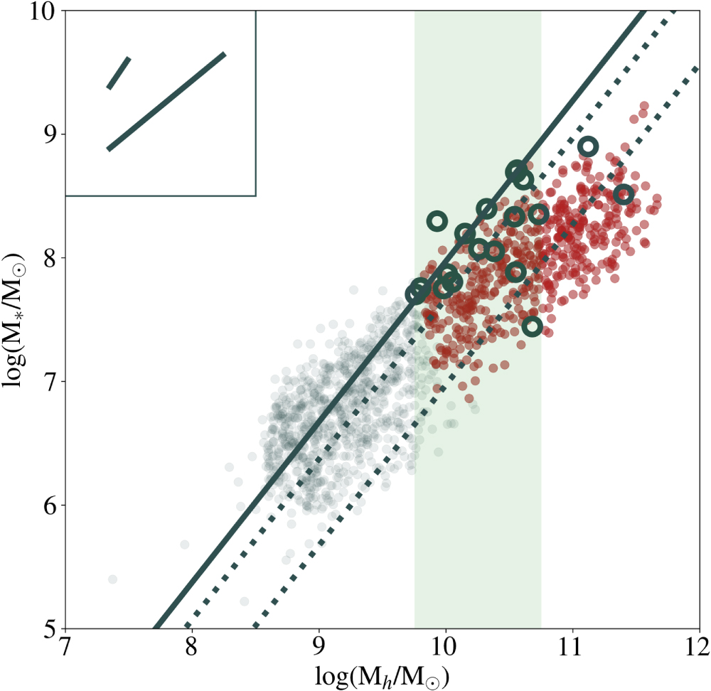
In Figure 10 we compare the stellar mass–halo mass (SMHM) relation for UDGs and other smaller low surface brightness galaxies in SMUDGes to the mean relation found using the same approach for the general dwarf galaxy population (Zaritsky & Behroozi 2023). The UDGs are offset from the mean relation in the sense that they are star-deficient at a given Mh . The magnitude of the effect is largest for those with the largest size or Mh . As we consider galaxies with lower values of Mh , the SMUDGes sources eventually merge onto the mean relation. On average, the offset for UDGs with 9.73 < log(Mh /M⊙) < 10.7 (the shaded region in Figure 10) is 0.61 ± 0.02 dex (a factor of ∼4), but for the most-massive UDGs, the integrated star formation efficiency is roughly an order of magnitude lower than for the general galaxy population. Over the full mass range of UDGs, we find an average factor of 7 deficiency. The range of Mh we find for UDGs, 1010 < Mh /M⊙ < 1011.5, is mostly in line with certain theoretical expectations (1010−1011 M⊙; Di Cintio et al. 2017; Rong et al. 2017) and consistent with limits from gravitational lensing (Sifón et al. 2018), providing some further encouragement for our mass estimates.
Figure 10. The SMHM relation for SMUDGes sources. The red, filled symbols represent UDGs (re ≥ 1.5 kpc), which correspond closely to a cut in Mh . The lighter colored points represent the SMUDGes that do not meet the UDG size criterion. The solid line represents the mean relation for a wide set of dwarf galaxies drawn from the literature (Zaritsky & Behroozi 2023). The dotted lines represent a decrease in the stellar mass by factors of 2 and 10. The large unfilled dark circles represent the results for a sample of UDGs with spectroscopically measured velocity dispersions and independent photometry. The shaded region highlights the range of Mh where we compare the samples in the text. The lines in the inset represent how an individual galaxy will move with a 10% and 100% error in the distance. Small errors move points along the published relation but significantly overestimating the distance moves points in the direction populated by the largest UDGs. The UDGs are relatively inefficient integrated star-forming galaxies at a given Mh . At a quantitative level, the results await further validation of the methodology for estimating σv and Mh .
Download figure:
Standard image High-resolution image
In the same figure we also plot the sample of UDGs that we used in Figure 5 to test the velocity dispersion estimates. Here we use the spectroscopic velocity dispersion measurements and the independent values of re , distance, and magnitudes provided by the source references and derive Mh as we do for our sample. Despite the fact that this is a much smaller sample and mean trends are more difficult to quantify, these points also preferentially fall below the fiducial SMHM relation. The offset within the shaded region in Figure 10 is not quite as large as for the SMUDGes sample in the same mass range (mean offset is 0.22 ± 0.10 dex, a factor of ∼1.7 deficient in stars in comparison to a factor of 4). We defined the shaded region to maximize the overlap between our sample and the literature sample in Mh and provide a fair baseline for comparison. For the entire literature sample, we find an average offset of 0.29 ± 0.10 dex.
An alternate interpretation, if one posits that galaxies have the same mean stellar to dark matter mass ratio, is that the dark matter profiles differ systematically between ‘normal’ galaxies and UDGs in this mass range, such that we are incorrectly estimating the masses for at least one of these two types of galaxies. However, the sense of the difference is that the UDGs would have to have a more concentrated dark matter profile than the normal galaxies, a trend which seems at odds with their larger sizes. We prefer the interpretation that the star formation efficiencies differ.
Although the results from our sample and the literature sample both suggest a deficit of stars in UDGs, the quantitative results disagree, suggesting the presence of systematic uncertainties. On our side of the equation, we face potential systematics in the estimation of the distances and velocity dispersions. We expect that 30% of the sample has incorrect distances (Section 4.1) and know that distance errors tend to scatter sources at an angle to the fiducial SMHM relation that is consistent with that seen in Figure 10 (Zaritsky & Behroozi2023). Furthermore, systematic differences in re measurements among samples can lead to offset differences. For example, if we reduce our measurements of re by 30%, we decrease the measured offset to our fiducial SMHM to 0.41 ± 0.02 dex, which is now roughly only 2σ discrepant with the literature value. On the literature side of the equation, observational biases (spectroscopy is most likely to succeed for UDGs with higher surface brightnesses or for star-forming UDGs exhibiting emission lines) could lead to unrepresentative samples that favor systems with higher relative stellar masses. Given the uncertainties in this discussion, we broadly claim that the stellar deficiency lies somewhere between a factor of 1.5–4 in the mass range of the comparison and 1.5–7 for the full UDG mass range.
There are various possible causes for the relative low integrated star formation efficiency in UDGs within the existing set of formation scenarios. For example, gas stripping would naturally lead to less star formation over the lifetime of the galaxy, and a high specific angular momentum could halt some gas from collapsing and reaching the densities required for star formation. The one set of models that can be excluded by this result is the set that explain UDGs solely by redistributing the stars to larger radii at late times. However, most models that invoke dynamical interactions as a key component of dwarf galaxy evolution suggest that a redistribution of stars occurs in conjunction with the loss of stars from the system (e.g., Peñarrubia et al. 2008; Tomozeiu et al. 2016; Carleton et al. 2019).
The most extreme offsets are at the largest masses. The estimates of Mh can surely be incorrect, but appear unlikely to be overestimated by a factor of 10. The agreement between the estimated and measured velocity dispersions shown in Figure 8 suggests that there is no large overall bias in the dispersion estimates, eliminating this specific issue as a concern. As mentioned previously, on further examination of Figure 8, there is some concern about a possible systematic failure of our dispersion estimates for log σv < 1.25, but this is not the regime of the most-massive UDGs, and the dispersion estimates agree well with measurements above log σv = 1.25. The previous discussion regarding NGC and the extrapolated total masses suggests similar concurrence with independent estimates (Figure 9).
Another concern is the effect of distance errors, which propagate into both M* and Mh . We show in Figure 10 the direction and amplitude of shifts due to 10% and 100% distance errors. For small errors, the points slide basically along the direction of the published relation and do not result in offsets from it. However, as the errors grow, the shift pushes the data away from the published relation in a manner consistent with what we find if many of our distances are gross overestimates. Of course, 100% errors fall into the category of catastrophic distance errors, and we only expect such errors for 30% the sample. If we remove the 30% of UDGs with the largest masses, the largest remaining UDG still has Mh > 1011 M⊙. For this mass, the offset from the fiducial SMHM relation is still about an order of magnitude. However, such errors may explain why there is a difference in the mean offset between the full sample and that composed of galaxies with spectroscopic distances and σv .
We could also be overestimating masses if the adopted potential profile is incorrect. However, by selecting a cuspy profile, NFW, we are likely to underestimate rather than overestimate the mass, as may indeed be the case for NGC 5846 UDG1. There are ways to contaminate the mass estimates, such as with the presence of a central massive black hole, but that contamination would have to be systemic and different in a relative sense to what is occurring in galaxies of similar stellar mass. Citing Occam’s razor, we conclude that UDGs are the relative star-deficient tail of the galaxy distribution at the corresponding values of Mh . This does not exclude the possibility that they are also the physically large tail of the population and that those two aspects are physically related.
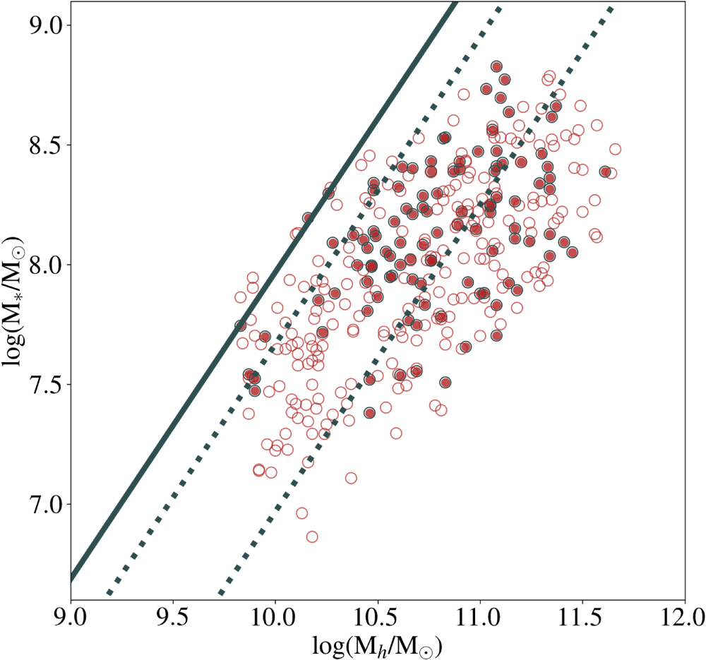
As a test of the effect of interactions and the role of local environment, we present the SMHM relation of UDGs separately for those in rich and poor environments as defined in Section 4.2 in Figure 11. There is no clear distinction between the two populations. Of course, absence of evidence is not evidence of absence. For example, the outer portions of the dark matter halo could have been stripped away in the subset of UDGs in high-density environments, and any gas reservoir may have been tidally or ram pressure stripped as well. Neither of these events would necessarily show up in our comparison. What the agreement between the two SMHM relations does demonstrate is that environment has not affected the structure within re sufficiently to differentially affect our estimates of σv and Mh . As such, we interpret the agreement to mean that dynamical processes are unlikely to affect re and hence to be directly related to the creation of UDGs. This conclusion is independently supported by the near linearity of the NUDG versus the halo mass relation from 1012–1015 M⊙ (e.g., Karunakaran & Zaritsky 2023), although we again stress that given the likely heterogeneous nature of the UDG populations, models that produce a variety of UDGs (e.g., Sales et al. 2020) may have enough flexibility to match these disparate observations. Our results at least present empirical benchmarks against which to test such models.
Figure 11. The SMHM relation for UDGs in poor and rich environments. The solid circles represent those UDGs in rich environments, and open circles represent those in poor ones, with environment defined as described in the text. The solid line represents the mean relation for the general population from Zaritsky & Behroozi (2023). The dotted lines represent a decrease in the stellar mass by factors of 2 and 10. The uncertainties due to distance errors are as shown in Figure 10.
Download figure:
Standard image High-resolution image
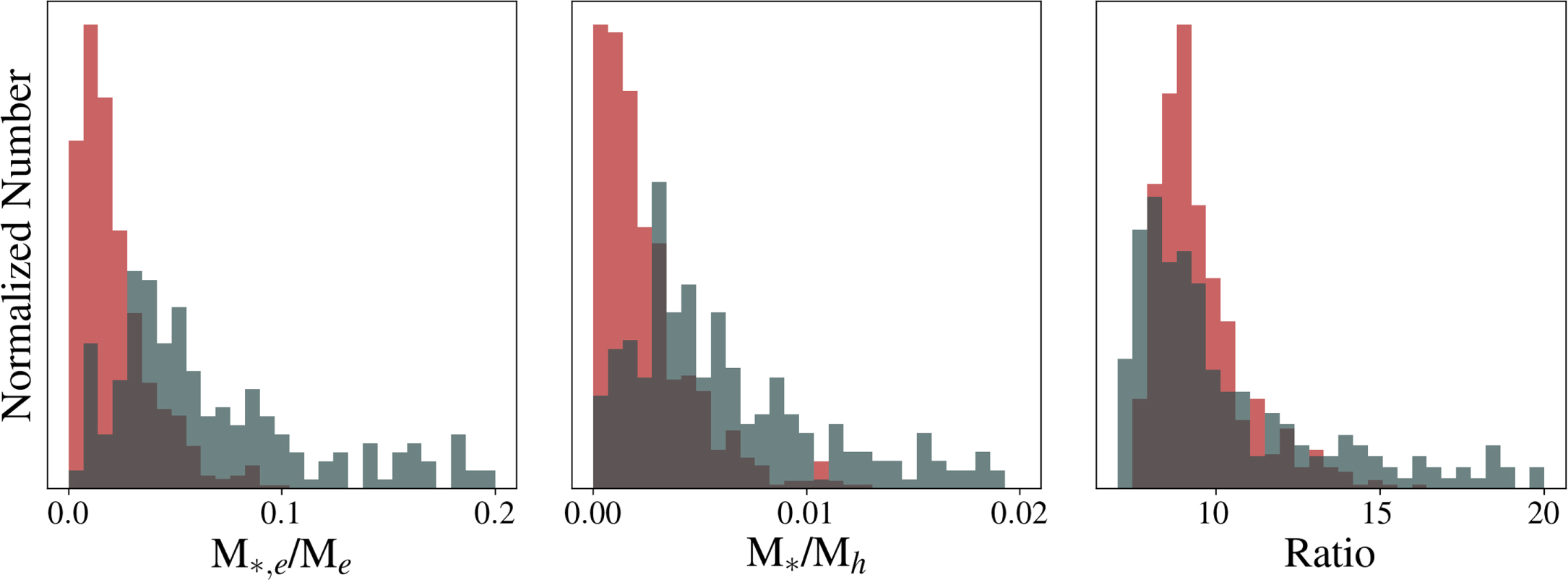
To assess whether UDGs are both star-deficient and "puffier," we compare the ratio of stellar to total mass within re , M*,e /Me , and within the virial radius, M*/Mh , for UDGs and the general galaxy population over a limited range of Mh (10 < Mh /M⊙ < 11.5). If UDGs are simply deficient in stars but have no structural differences, then these ratios should change by the same factor within re and r200. We present that comparison in Figure 12.
Figure 12. Comparison of UDGs (red) and the general galaxy population (gray) with 10 < Mh /M⊙ < 11.5. The first panel shows the stellar mass to total mass ratio within re , while the second shows the same ratio for the halo radius, rh . Finally, the third panel shows the distribution of the ratio of these two quantities. Smaller ratios indicate a lower concentration of stars relative to dark matter.
Download figure:
Standard image High-resolution image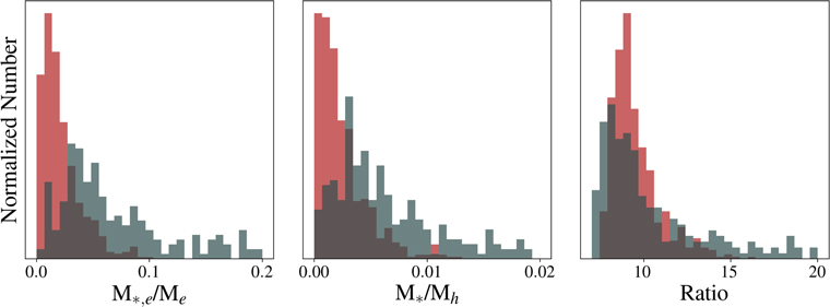
The distributions of M*,e /Me and M*/Mh are quite similar, and that impression is confirmed in the third panel, which plots the ratio of the value at re to that at rh for the two galaxy populations. The UDG population does not exhibit significantly different behavior, suggesting that size differences in the stellar component are not a primary factor. In fact, the ratio peaks at slightly smaller values for the general population, probably due to the larger relative contribution of the stellar mass within re in the general galaxy population. We conclude that whatever processes are involved in forming a UDG, they lead primarily to a decrease in the integrated star formation rate in galaxies of comparable total mass.
6. Summary
In this last of the SMUDGes catalog papers, we present the full UDG candidate catalog drawn from the Legacy Survey DR9 release (Dey et al. 2019) following our described procedure and selection. The catalog contains 7070 candidates with μ0,g ≥ 24 mag arcsec−2 and re ≥ 5.3′′ as measured using single Sérsic models and our particular masking algorithms. After visual examination, we consider 265 of these to be poor candidates and flag them as such. Using the parameters of each candidate, we estimate and tabulate the completeness fraction across the full survey for similar galaxies using artificial source simulations. The catalog is highly incomplete for sources with re ≳ 20′′ due to our choice of filtering. The mean overall completeness for galaxies like those already in the catalog is close to 50%.
We estimate and tabulate distances for a subsample of 1525 candidates using the distance-by-association technique described in Paper III, associating candidates projected onto the Coma, Fornax, and Virgo clusters with those clusters, and using the Kadowaki et al. (2021) compilation of spectroscopic redshifts. Because of the overrepresentation of Virgo and Fornax galaxies in this list, the fraction of UDGs (re ≥ 1.5 kpc) in this list is small (40%) resulting in a total of 585 UDGs, but they are distributed across the sky. They have total magnitudes typically in the range −17 ≲ Mr ≲ − 14 and are typically red, g − r ∼ 0.6, although there is a blue population that extends to g − r ∼ 0.1.
We estimate and tabulate total masses, Mh , using an approach presented by Zaritsky & Behroozi (2023). Although the approach is speculative for UDGs and needs further validation, it provides a way forward at the current time. It provides accurate (to within 25%) mass estimates in comparison to those from the number of globular clusters for a sample of six UDGs (Saifollahi et al. 2022). We find that UDGs have total masses in the range of 1010 ≲ Mh /M⊙ ≲ 1011.5. Comparing the SMHM relation of UDGs to that of the general population over the same range of Mh from Zaritsky & Behroozi (2023), we find that UDGs are increasingly star-deficient with increasing Mh . The average deficit of stars varies as a function of galaxy size and total mass and likely lies somewhere between a factor 1.5 and 7 for the UDG sample as a whole.
We conclude that whatever processes are involved in forming UDGs, they do not simply reorganize the stars to larger radii but instead result in a measurable decrease, up to an order of magnitude, in the integrated star formation rates relative to other galaxies of the same total mass (1010 < Mh /M⊙ < 1011.5). This deficiency does not have a detectable environmental dependence.
Acknowledgments
D.Z., R.D., J.K., D.J.K., and H.Z. acknowledge financial support from NSF AST-1713841 and AST-2006785. D.Z. thanks the Astronomy Department at Columbia University for hosting him during his sabbatical. A.D.’s research is supported by NOIRLab. K.S. acknowledges funding from the Natural Sciences and Engineering Research Council of Canada (NSERC). A.K. acknowledges financial support from the grant CEX2021-001131-S funded by MCIN/AEI/ 10.13039/501100011033 and from the grant POSTDOC_21_00845 funded by the Economic Transformation, Industry, Knowledge and Universities Council of the Regional Government of Andalusia. An allocation of computer time from the UA Research Computing High Performance Computing (HPC) at the University of Arizona and the prompt assistance of the associated computer support group is gratefully acknowledged.
This research has made use of the NASA/IPAC Extragalactic Database (NED), which is operated by the Jet Propulsion Laboratory, California Institute of Technology, under contract with NASA.
The Legacy Surveys consist of three individual and complementary projects: the Dark Energy Camera Legacy Survey (DECaLS; Proposal ID No. 2014B-0404; PIs: David Schlegel and Arjun Dey), the Beijing–Arizona Sky Survey (BASS; NOAO Prop. ID No. 2015A-0801; PIs: Zhou Xu and Xiaohui Fan), and the Mayall z-band Legacy Survey (MzLS; Prop. ID No. 2016A-0453; PI: Arjun Dey). DECaLS, BASS, and MzLS together include data obtained, respectively, at the Blanco telescope, Cerro Tololo Inter-American Observatory, NSF’s NOIRLab; the Bok telescope, Steward Observatory, University of Arizona; and the Mayall telescope, Kitt Peak National Observatory, NOIRLab. Pipeline processing and analyses of the data were supported by NOIRLab and the Lawrence Berkeley National Laboratory (LBNL). The Legacy Surveys project is honored to be permitted to conduct astronomical research on Iolkam Du’ag (Kitt Peak), a mountain with particular significance to the Tohono O’odham Nation.
NOIRLab is operated by the Association of Universities for Research in Astronomy (AURA) under a cooperative agreement with the National Science Foundation. LBNL is managed by the Regents of the University of California under contract to the U.S. Department of Energy.
This project used data obtained with the Dark Energy Camera (DECam), which was constructed by the Dark Energy Survey (DES) collaboration. Funding for the DES Projects has been provided by the U.S. Department of Energy, the U.S. National Science Foundation, the Ministry of Science and Education of Spain, the Science and Technology Facilities Council of the United Kingdom, the Higher Education Funding Council for England, the National Center for Supercomputing Applications at the University of Illinois at Urbana-Champaign, the Kavli Institute of Cosmological Physics at the University of Chicago, Center for Cosmology and Astro-Particle Physics at the Ohio State University, the Mitchell Institute for Fundamental Physics and Astronomy at Texas A&M University, Financiadora de Estudos e Projetos, Fundacao Carlos Chagas Filho de Amparo, Financiadora de Estudos e Projetos, Fundacao Carlos Chagas Filho de Amparo a Pesquisa do Estado do Rio de Janeiro, Conselho Nacional de Desenvolvimento Cientifico e Tecnologico and the Ministerio da Ciencia, Tecnologia e Inovacao, the Deutsche Forschungsgemeinschaft and the Collaborating Institutions in the Dark Energy Survey. The Collaborating Institutions are Argonne National Laboratory, the University of California at Santa Cruz, the University of Cambridge, Centro de Investigaciones Energeticas, Medioambientales y Tecnologicas-Madrid, the University of Chicago, University College London, the DES-Brazil Consortium, the University of Edinburgh, the Eidgenossische Technische Hochschule (ETH) Zurich, Fermi National Accelerator Laboratory, the University of Illinois at Urbana-Champaign, the Institut de Ciencies de l’Espai (IEEC/CSIC), the Institut de Fisica dAltes Energies, Lawrence Berkeley National Laboratory, the Ludwig Maximilians Universitat Munchen and the associated Excellence Cluster Universe, the University of Michigan, NSFs NOIRLab, the University of Nottingham, the Ohio State University, the University of Pennsylvania, the University of Portsmouth, SLAC National Accelerator Laboratory, Stanford University, the University of Sussex, and Texas A&M University.
BASS is a key project of the Telescope Access Program (TAP), which has been funded by the National Astronomical Observatories of China, the Chinese Academy of Sciences (the Strategic Priority Research Program "The Emergence of Cosmological Structures" grant No. XDB09000000), and the Special Fund for Astronomy from the Ministry of Finance. BASS is also supported by the External Cooperation Program of Chinese Academy of Sciences (grant No. 114A11KYSB20160057), and Chinese National Natural Science Foundation (grant Nos. 12120101003 and 11433005).
The Legacy Survey team makes use of data products from the Near-Earth Object Wide-field Infrared Survey Explorer (NEOWISE), which is a project of the Jet Propulsion Laboratory/California Institute of Technology. NEOWISE is funded by the National Aeronautics and Space Administration.
The Legacy Surveys imaging of the DESI footprint is supported by the Director, Office of Science, Office of High Energy Physics of the U.S. Department of Energy under contract No. DE-AC02-05CH1123, by the National Energy Research Scientific Computing Center, a DOE Office of Science User Facility under the same contract; and by the U.S. National Science Foundation, Division of Astronomical Sciences under contract No. AST-0950945 to NOAO.
Facilities: Blanco - Cerro Tololo Inter-American Observatory's 4 meter Blanco Telescope, Mayall - Kitt Peak National Observatory's 4 meter Mayall Telescope, Bok - Steward Observatory 2.3 meter Bok Telescope.
Software: Astropy (Astropy Collaboration et al. 2013, 2018), astroquery (Ginsburg et al. 2019), GALFIT (Peng et al. 2002), keras (https://github.com/keras-team/keras), lmfit (Newville et al. 2014), Matplotlib (Hunter 2007), NumPy (van der Walt et al. 2011), pandas (McKinney 2010), sep (Barbary 2016), Source Extractor (Bertin & Arnouts 1996), SciPy (Oliphant 2007; Millman & Aivazis 2011), SWarp (Bertin et al.2002).