This site needs JavaScript to work properly. Please enable it to take advantage of the complete set of features!
Skip to main page content
U.S. flag

An official website of the United States government

Dot gov

The .gov means it’s official.
Federal government websites often end in .gov or .mil. Before sharing sensitive information, make sure you’re on a federal government site.

Https

The site is secure.
The https:// ensures that you are connecting to the official website and that any information you provide is encrypted and transmitted securely.

NIH NLM Logo
Log in
Access keys NCBI Homepage MyNCBI Homepage Main Content Main Navigation
. 2023 Dec 13;21(12):e3002366.
doi: 10.1371/journal.pbio.3002366. eCollection 2023 Dec.

Many but not all deep neural network audio models capture brain responses and exhibit correspondence between model stages and brain regions

Affiliations

Many but not all deep neural network audio models capture brain responses and exhibit correspondence between model stages and brain regions

Greta Tuckute et al. PLoS Biol. .

Abstract

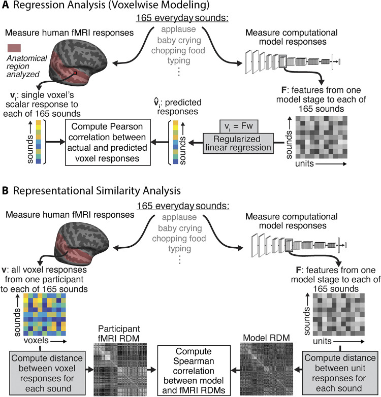
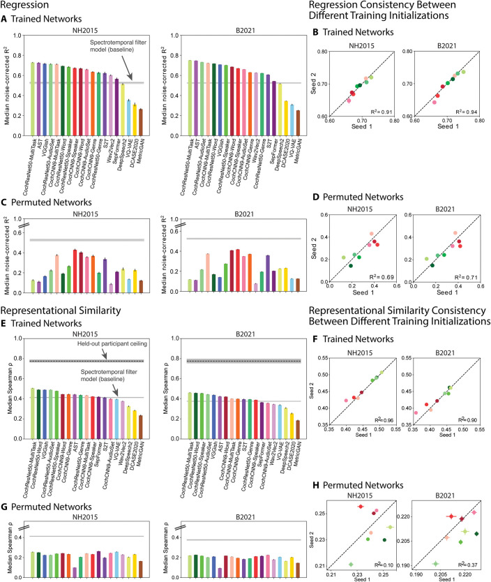
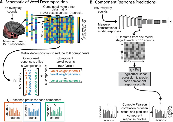
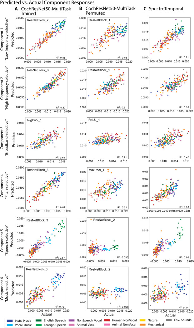
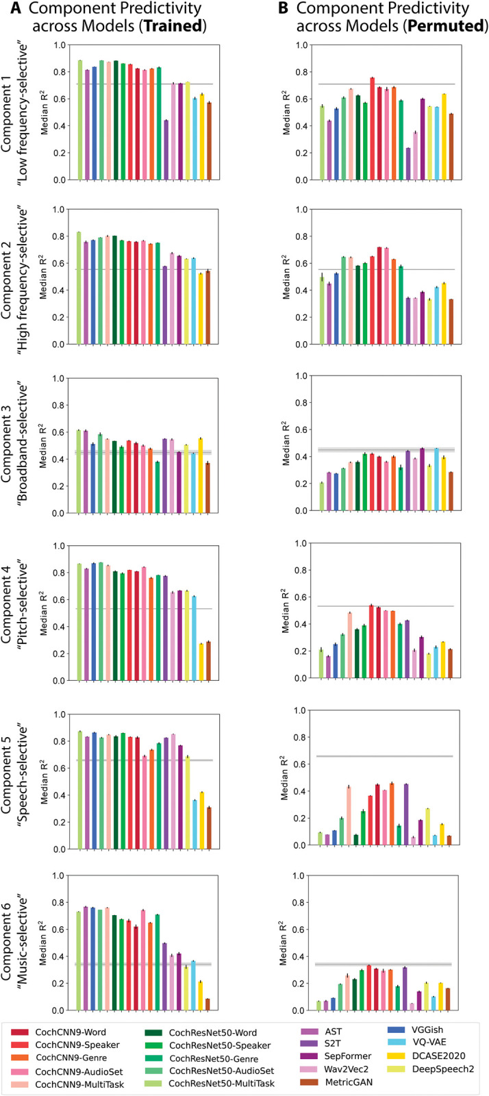
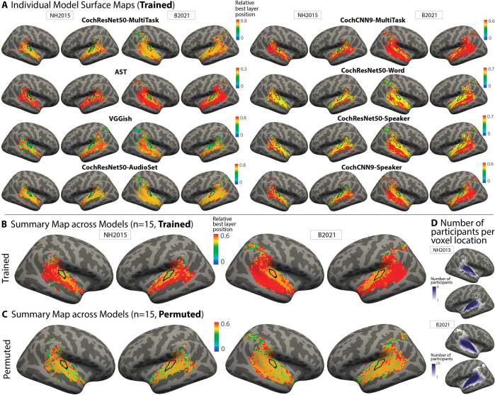
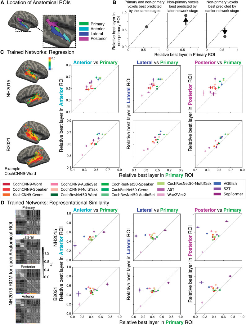
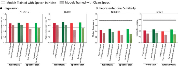
Models that predict brain responses to stimuli provide one measure of understanding of a sensory system and have many potential applications in science and engineering. Deep artificial neural networks have emerged as the leading such predictive models of the visual system but are less explored in audition. Prior work provided examples of audio-trained neural networks that produced good predictions of auditory cortical fMRI responses and exhibited correspondence between model stages and brain regions, but left it unclear whether these results generalize to other neural network models and, thus, how to further improve models in this domain. We evaluated model-brain correspondence for publicly available audio neural network models along with in-house models trained on 4 different tasks. Most tested models outpredicted standard spectromporal filter-bank models of auditory cortex and exhibited systematic model-brain correspondence: Middle stages best predicted primary auditory cortex, while deep stages best predicted non-primary cortex. However, some state-of-the-art models produced substantially worse brain predictions. Models trained to recognize speech in background noise produced better brain predictions than models trained to recognize speech in quiet, potentially because hearing in noise imposes constraints on biological auditory representations. The training task influenced the prediction quality for specific cortical tuning properties, with best overall predictions resulting from models trained on multiple tasks. The results generally support the promise of deep neural networks as models of audition, though they also indicate that current models do not explain auditory cortical responses in their entirety.


Conflict of interest statement

The authors have declared that no competing interests exist.

Figures

Fig 1
Fig 1. Analysis method.
(A) Regression analysis (voxelwise modeling). Brain activity of human participants (n = 8, n = 20) was recorded with fMRI while they listened to a set of 165 natural sounds. Data were taken from 2 previous publications [50,51]. We then presented the same set of 165 sounds to each model, measuring the time-averaged unit activations from each model stage in response to each sound. We performed an encoding analysis where voxel activity was predicted by a regularized linear model of the DNN activity. We modeled each voxel as a linear combination of model units from a given model stage, estimating the linear transform with half (n = 83) the sounds and measuring the prediction quality by correlating the empirical and predicted response to the left-out sounds (n = 82) using the Pearson correlation. We performed this procedure for 10 random splits of the sounds. Figure adapted from Kell and colleagues’ article [31]. (B) Representational similarity analysis. We used the set of brain data and model activations described for the voxelwise regression modeling. We constructed a representational dissimilarity matrix (RDM) from the fMRI responses by computing the distance (1−Pearson correlation) between all voxel responses to each pair of sounds. We similarly constructed an RDM from the unit responses from a model stage to each pair of sounds. We measured the Spearman correlation between the fMRI and model RDMs as the metric of model-brain similarity. When reporting this correlation from a best model stage, we used 10 random splits of sounds, choosing the best stage from the training set of 83 sounds and measuring the Spearman correlation for the remaining set of 82 test sounds. The fMRI RDM is the average RDM across all participants for all voxels and all sounds in NH2015. The model RDM is from an example model stage (ResNetBlock_2 of the CochResNet50-MultiTask network).
Fig 2
Fig 2. Evaluation of overall model-brain similarity.
(A) Using regression, explained variance was measured for each voxel, and the aggregated median variance explained was obtained for the best-predicting stage for each model, selected using independent data. Grey line shows variance explained by the SpectroTemporal baseline model. Colors indicate the nature of the model architecture: CochCNN9 architectures in shades of red, CochResNet50 architectures in shades of green, Transformer architectures in shades of violet (AST, Wav2Vec2, S2T, SepFormer), recurrent architectures in shades of yellow (DCASE2020, DeepSpeech2), other convolutional architectures in shades of blue (VGGish, VQ-VAE), and miscellaneous in brown (MetricGAN). Error bars are within-participant SEM. Error bars are smaller for the B2021 dataset because of the larger number of participants (n = 20 vs. n = 8). For both datasets, most trained models outpredict the baseline model. (B) We trained the in-house models from 2 different random seeds. The median variance explained for the first- and second-seed models are plotted on the x- and y-axes, respectively. Each data point represents a model using the same color scheme as in panel A. (C, D) Same analysis as in panels A and B but for the control networks with permuted weights. All permuted models produce worse predictions than the baseline. (E) Representational similarity between all auditory cortex fMRI responses and the trained computational models. The models and colors are the same as in panel A. The dashed black line shows the noise ceiling measured by comparing one participant’s RDM with the average of the RDMs from the other participants (we plot the noise ceiling rather than noise correcting as in the regression analyses in order to be consistent with what is standard for each analysis). Error bars are within-participant SEM. As in the regression analysis, many of the trained models exhibit RDMs that are more correlated with the human RDM than is the baseline model’s RDM. (F) The Spearman correlation between the model and fMRI RDMs for 2 different seeds of the in-house models. The results for the first and second seeds are plotted on the x- and y-axes, respectively. Each data point represents a model using the same color scheme as in panel E. (G, H) Same analysis as in panels E and F but with the control networks with permuted weights. RDMs for all permuted models are less correlated with the human RDM compared to the baseline model’s correlation with the human RDM. Data and code with which to reproduce results are available at https://github.com/gretatuckute/auditory_brain_dnn.
Fig 3
Fig 3. Component decomposition of fMRI responses.
(A) Voxel component decomposition method. The voxel responses of a set of participants are approximated as a linear combination of a small number of component response profiles. The solution to the resulting matrix factorization problem is constrained to maximize a measure of the non-Gaussianity of the component weights. Voxel responses in auditory cortex to natural sounds are well accounted for by 6 components. Figure adapted from Norman-Haignere and colleagues’ article [50]. (B) We generated model predictions for each component’s response using the same approach used for voxel responses, in which the model unit responses were combined to best predict the component response, with explained variance measured in held-out sounds (taking the median of the explained variance values obtained across train/test cross-validation splits).
Fig 4
Fig 4. Example model predictions for 6 components of fMRI responses to natural sounds.
(A) Predictions of the 6 components by a trained DNN model (CochResNet50-MultiTask). Each data point corresponds to a single sound from the set of 165 natural sounds. Data point color denotes the sound’s semantic category. Model predictions were made from the model stage that best predicted a component’s response. The predicted response is the average of the predictions for a sound across the test half of 10 different train-test splits (including each of the splits for which the sound was present in the test half). (B) Predictions of the 6 components by the same model used in (A) but with permuted weights. Predictions are substantially worse than for the trained model, indicating that task optimization is important for obtaining good predictions, especially for components 4–6. (C) Predictions of the 6 components by the SpectroTemporal model. Predictions are substantially worse than for the trained model, particularly for components 4–6. Data and code with which to reproduce results are available at https://github.com/gretatuckute/auditory_brain_dnn.
Fig 5
Fig 5. Summary of model predictions of fMRI response components.
(A) Component response variance explained by each of the trained models. Model ordering is the same as that in Fig 2A for ease of comparison. Variance explained was obtained from the best-predicting stage of each model for each component, selected using independent data. Error bars are SEM over iterations of the model stage selection procedure (see Methods; Component modeling). See S3 Fig for a comparison of results for models trained with different random seeds (results were overall similar for different seeds). (B) Component response variation explained by each of the permuted models. The trained models (both in-house and external), but not the permuted models, tend to outpredict the SpectroTemporal baseline for all components, but the effect is most pronounced for components 4–6. Data and code with which to reproduce results are available at https://github.com/gretatuckute/auditory_brain_dnn.
Fig 6
Fig 6. Surface maps of best-predicting model stage.
(A) To investigate correspondence between model stages and brain regions, we plot the model stage that best predicts each voxel as a surface map (FsAverage) (median best stage across participants). We assigned each model stage a position index between 0 and 1 (using minmax normalization such that the first stage is assigned a value of 0 and the last stage a value of 1). We show this map for the 8 best-predicting models as evaluated by the median noise-corrected R2 plotted in Fig 2A (see S4 Fig for maps from other models). The color scale limits were set to extend from 0 to the stage beyond the most common best stage (across voxels). We found that setting the limits in this way made the variation across voxels in the best stage visible by not wasting dynamic range on the deep model stages, which were almost never the best-predicting stage. Because the relative position of the best-predicting stage varied across models, the color bar scaling varies across models. For both datasets, middle stages best predict primary auditory cortex, while deep stages best predict non-primary cortex. We note that the B2021 dataset contained voxel responses in parietal cortex, some of which passed the reliability screen. We have plotted a best-predicting stage for these voxels in these maps for consistency with voxel inclusion criteria in the original publication [51], but note that these voxels only passed the reliability screen in a few participants (see panel D) and that the variance explained for these voxels was low, such that the best-predicting stage is not very meaningful. (B) Best-stage map averaged across all models that produced better predictions than the baseline SpectroTemporal model. The map plots the median value across models and thus is composed of discrete color values. The thin black outline plots the borders of an anatomical ROI corresponding to primary auditory cortex. (C) Best-stage map for the same models as in panel B, but with permuted weights. (D) Maps showing the number of participants per voxel location on the FsAverage surface for both datasets (1–8 participants for NH2015; 1–20 participants for B2021). Darker colors denote a larger number of participants per voxel. Because we only analyzed voxels that passed a reliability threshold, some locations only passed the threshold in a few participants. Note also that the regions that were scanned were not identical in the 2 datasets. Data and code with which to reproduce results are available at https://github.com/gretatuckute/auditory_brain_dnn.
Fig 7
Fig 7. Nearly all DNN models exhibit stage-region correspondence.
(A) Anatomical ROIs for analysis. ROIs were taken from a previous study [51], in which they were derived by pooling ROIs from the Glasser anatomical parcellation [67]. (B) To summarize the model-stage-brain-region correspondence across models, we obtained the median best-predicting stage for each model within the 4 anatomical ROIs from A: primary auditory cortex (x-axis in each plot in C and D) and anterior, lateral, and posterior non-primary regions (y-axes in C and D) and averaged across participants. (C) We performed the analysis on each of the 2 fMRI datasets, including each model that outpredicted the baseline model in Fig 2 (n = 15 models). Each data point corresponds to a model, with the same color correspondence as in Fig 2. Error bars are within-participant SEM. The non-primary ROIs are consistently best predicted by later stages than the primary ROI. (D) Same analysis as (C) but with the best-matching model stage determined by correlations between the model and ROI representational dissimilarity matrices. RDMs for each anatomical ROI (left) are grouped by sound category, indicated by colors on the left and bottom edges of each RDM (same color-category correspondence as in Fig 4). Higher-resolution fMRI RDMs for each ROI including the name of each sound are provided in S1 Fig. Data and code with which to reproduce results are available at https://github.com/gretatuckute/auditory_brain_dnn.
Fig 8
Fig 8. Model predictions of brain responses are better for models trained in background noise.
(A) Effect of noise in training on model-brain similarity assessed via regression. Using regression, explained variance was measured for each voxel and the aggregated median variance explained was obtained for the best-predicting stage for each model, selected using independent data. Grey line shows variance explained by the SpectroTemporal baseline model. Colors indicate the nature of the model architecture with CochCNN9 architectures in shades of red, and CochResNet50 architectures in shades of green. Models trained in the presence of background noise are shown in the same color scheme as in Fig 2; models trained with clean speech are shown with hashing. Error bars are within-participant SEM. For both datasets, the models trained in the presence of background noise exhibit higher model-brain similarity than the models trained without background noise. (B) Effect of noise in training on model-brain representational similarity. Same conventions as (A), except that the dashed black line shows the noise ceiling measured by comparing one participant’s RDM with the average of the RDMs from each of the other participants. Error bars are within-participant SEM. Data and code with which to reproduce results are available at https://github.com/gretatuckute/auditory_brain_dnn.
Fig 9
Fig 9. Training task modulates model predictions.
(A) Component response variance explained by each of the trained in-house models. Predictions are shown for components 4–6 (pitch-selective, speech-selective, and music-selective, respectively). The in-house models were trained separately on each of 4 tasks as well as on 3 of the tasks simultaneously, using 2 different architectures. Explained variance was measured for the best-predicting stage of each model for each component selected using independent data. Error bars are SEM over iterations of the model stage selection procedure (see Methods; Component modeling). Grey line plots the variance explained by the SpectroTemporal baseline model. (B) Scatter plots of in-house model predictions for pairs of components. The upper panel shows the variance explained for component 5 (speech-selective) vs. component 6 (music-selective), and the lower panel shows component 6 (music-selective) vs. component 4 (pitch-selective). Symbols denote the training task. In the left panel, the 4 models trained on speech-related tasks are furthest from the diagonal, indicating good predictions of speech-selective tuning at the expense of those for music-selective tuning. In the right panel, the models trained on AudioSet are set apart from the others in their predictions of both the pitch-selective and music-selective components. Error bars are smaller than the symbol width (and are provided in panel A) and so are omitted for clarity. Data and code with which to reproduce results are available at https://github.com/gretatuckute/auditory_brain_dnn.

References

    1. Lehky SR, Sejnowski TJ. Network model of shape-from-shading: neural function arises from both receptive and projective fields. Nature. 1988. Jun;333(6172):452–454. doi: 10.1038/333452a0 - DOI - PubMed
    1. Zipser D, Andersen RA. A back-propagation programmed network that simulates response properties of a subset of posterior parietal neurons. Nature. 1988. Feb;331(6158):679–684. doi: 10.1038/331679a0 - DOI - PubMed
    1. Marblestone AH, Wayne G, Kording KP. Toward an integration of deep learning and neuroscience. Front Comput Neurosci [Internet]. 2016. Sep 14 [cited 2022 Feb 8];10. Available from: http://journal.frontiersin.org/Article/10.3389/fncom.2016.00094/abstract - DOI - PMC - PubMed
    1. Richards BA, Lillicrap TP, Beaudoin P, Bengio Y, Bogacz R, Christensen A, et al.. A deep learning framework for neuroscience. Nat Neurosci. 2019. Nov;22(11):1761–1770. doi: 10.1038/s41593-019-0520-2 - DOI - PMC - PubMed
    1. Kell AJE, McDermott JH. Deep neural network models of sensory systems: windows onto the role of task constraints. Curr Opin Neurobiol. 2019. Apr;55:121–132. doi: 10.1016/j.conb.201902003 - DOI - PubMed
Cite

AltStyle によって変換されたページ (->オリジナル) /