This site needs JavaScript to work properly. Please enable it to take advantage of the complete set of features!
Skip to main page content
U.S. flag

An official website of the United States government

Dot gov

The .gov means it’s official.
Federal government websites often end in .gov or .mil. Before sharing sensitive information, make sure you’re on a federal government site.

Https

The site is secure.
The https:// ensures that you are connecting to the official website and that any information you provide is encrypted and transmitted securely.

NIH NLM Logo
Log in
Access keys NCBI Homepage MyNCBI Homepage Main Content Main Navigation
. 2023 Mar 1;14(1):1155.
doi: 10.1038/s41467-023-36796-3.

Spatially informed clustering, integration, and deconvolution of spatial transcriptomics with GraphST

Affiliations

Spatially informed clustering, integration, and deconvolution of spatial transcriptomics with GraphST

Yahui Long et al. Nat Commun. .

Abstract

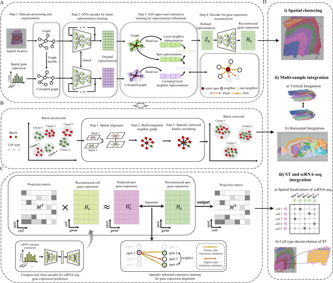
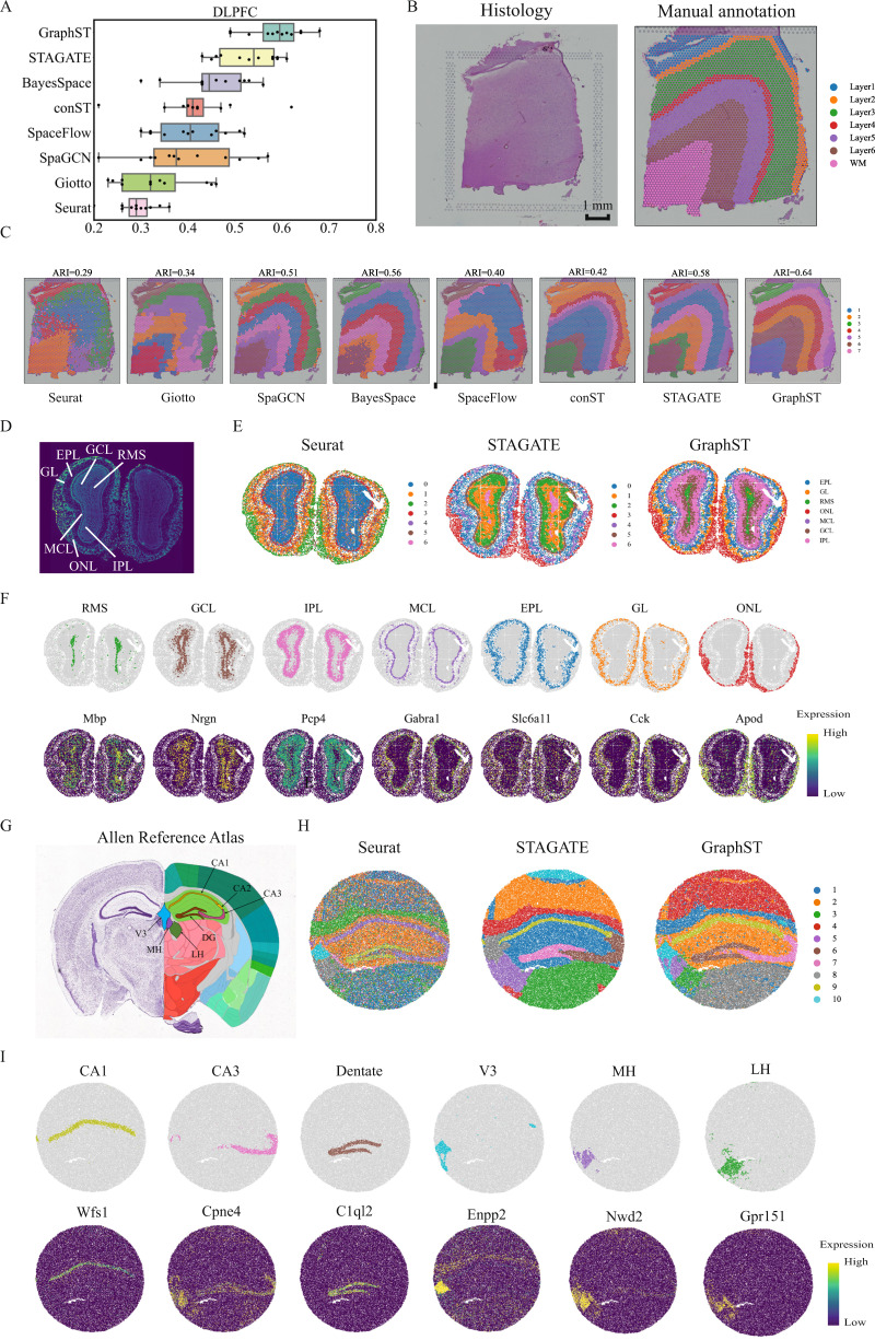
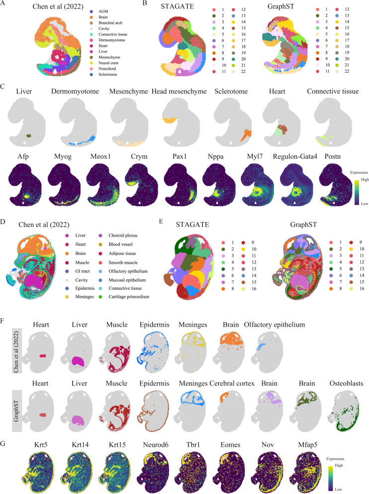
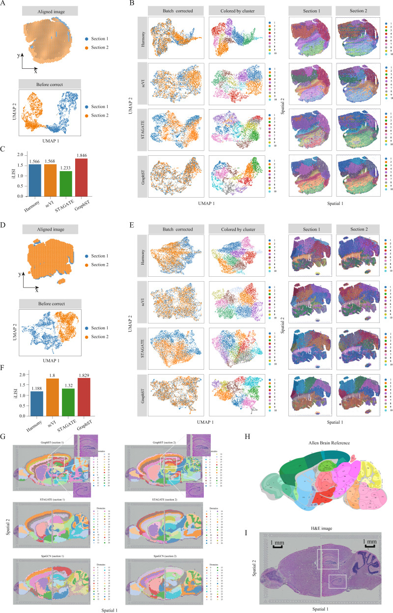
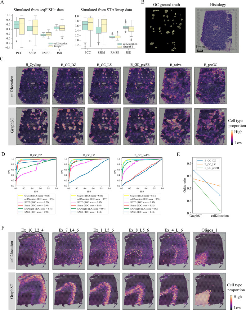
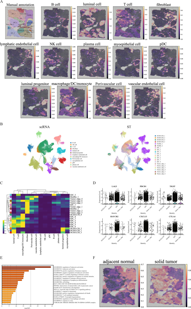
Spatial transcriptomics technologies generate gene expression profiles with spatial context, requiring spatially informed analysis tools for three key tasks, spatial clustering, multisample integration, and cell-type deconvolution. We present GraphST, a graph self-supervised contrastive learning method that fully exploits spatial transcriptomics data to outperform existing methods. It combines graph neural networks with self-supervised contrastive learning to learn informative and discriminative spot representations by minimizing the embedding distance between spatially adjacent spots and vice versa. We demonstrated GraphST on multiple tissue types and technology platforms. GraphST achieved 10% higher clustering accuracy and better delineated fine-grained tissue structures in brain and embryo tissues. GraphST is also the only method that can jointly analyze multiple tissue slices in vertical or horizontal integration while correcting batch effects. Lastly, GraphST demonstrated superior cell-type deconvolution to capture spatial niches like lymph node germinal centers and exhausted tumor infiltrating T cells in breast tumor tissue.


Conflict of interest statement

The authors declare no competing interests.

Figures

Fig. 1
Fig. 1. Overview of GraphST.
A GraphST takes as inputs the preprocessed spatial gene expressions and neighborhood graph constructed using spot coordinates (x,y). Latent representation Zs is first learned using our graph self-supervised contrastive learning to preserve the informative features from the gene expression profiles, spatial location information, and local context information. This is then reversed back into the original feature space to reconstruct the gene expression matrix Hs. B The analysis workflow for spatial batch effect correction by GraphST. The first step is to align the H&E images of two or more samples, followed by shared neighborhood graph construction, where both intra- and inter-sample neighbors are considered. This provides the possibility for feature smoothing. Finally, sample batch effects are implicitly corrected by smoothing features across samples with GraphST. C With the reconstructed spatial gene expression Hs and the refined scRNA-seq feature matrix Hc derived from an unsupervised auto-encoder, a cell-to-spot mapping matrix M is trained via a spatially informed contrastive learning mechanism where the similarities of positive pairs (i.e., spatially adjacent spot pairs) are maximized, and those of negative pairs (i.e., spatially nonadjacent spot pairs) are minimized. D The outputs Hs and M of GraphST can be utilized for spatial clustering, multiple ST data integration, and ST and scRNA-seq data integration.
Fig. 2
Fig. 2. GraphST clustering improves the identification of tissue structures in the human dorsolateral prefrontal cortex (DLPFC), mouse olfactory bulb, and mouse hippocampus tissue.
A Boxplots of adjusted rand index (ARI) scores of the eight methods applied to the 12 DLPFC slices. In the boxplot, the center line denotes the median, box limits denote the upper and lower quartiles, and whiskers denote the ×ばつ interquartile range. B H&E image and manual annotation from the original study. C Clustering results by nonspatial and spatial methods, Seurat, Giotto, SpaGCN, BayesSpace, SpaceFlow, conST, STAGATE, and GraphST on slice 151673 of the DLPFC dataset. Manual annotations and clustering results of the other DLPFC slices are shown in Supplementary Fig. S1. D Laminar organization of the mouse olfactory bulb annotated using the DAPI-stained image. E Spatial domains identified by Seurat, STAGATE, and GraphST in the mouse olfactory bulb Stereo-seq data. F Visualization of the spatial domains identified by GraphST and the corresponding marker gene expressions. The identified domains are aligned with the annotated laminar organization of the mouse olfactory bulb. G Allen Mouse Brain Atlas with the hippocampus region annotated. H Spatial domains identified by Seurat, STAGATE, and GraphST in mouse hippocampus tissue acquired with Slide-seqV2. I Visualization of the spatial domains identified by GraphST and the corresponding marker gene expressions. The identified domains are aligned with the annotated hippocampus region of the Allen Mouse Brain Atlas.
Fig. 3
Fig. 3. GraphST enables accurate identification of different organs in the Stereo-seq mouse embryo.
A Tissue domain annotations of the E9.5 mouse embryo data taken from the original Stereo-seq study wherein the clusters were first identified using Leiden clustering from SCANPY and then annotated using differentially expressed genes. B Clustering results of STAGATE and GraphST on the E9.5 mouse embryo data. C Visualization of selected spatial domains identified by GraphST and the corresponding marker gene expressions. D Tissue domain annotations of the E14.5 mouse embryo data obtained from the original Stereo-seq study. E Clustering results by STAGATE and GraphST on the E14.5 mouse embryo. F Visualization of selected spatial domains identified by the original Stereo-seq study and GraphST, respectively. G Visualization of marker gene expressions supporting the identified domains.
Fig. 4
Fig. 4. GraphST enables accurate vertical and horizontal integrations of ST data on mouse breast cancer and mouse brain anterior and posterior data, respectively.
A First set of mouse breast cancer sample images aligned with the PASTE algorithm and plotted before batch effect correction. B UMAP plots after batch effect correction and spatial clustering results from Harmony, scVI, STAGATE, and GraphST. Spots in the second column are colored according to the spatial domains identified by the respective clustering methods. C Barplots of iLISI metric for batch correction results from different methods on the first set of samples. D Second set of mouse breast cancer sample images aligned and UMAP plot before batch effect correction. E UMAP plots after batch effect correction and the spatial clusters detected by Harmony, scVI, STAGATE, and GraphST on sections 1 and 2, respectively. Similarly, spots in the second column are colored according to the spatial domains identified by the respective methods. F Barplots of iLISI metric for batch correction results from different methods on the second set of samples. G Horizontal integration results with two mouse brain samples, of which each consists of anterior and posterior brain sections. Top: spatial joint domains identified by GraphST on sections 1 and 2. Middle: spatial joint domains identified by STAGATE. Bottom: spatial joint domains identified by SpaGCN. H Annotated brain section image from Allen Mouse Brain Atlas for reference. I H&E image of mouse brain anterior and posterior.
Fig. 5
Fig. 5. Comparing the accuracy of GraphST with top deconvolution method cell2location in predicting spatial distributions of scRNA-seq data with simulated data, human lymph node, and the slice 151673 of DLPFC.
A Boxplots of PCC, SSIM, RMSE, and JSD metrics for cell2location and GraphST results on simulated data created from seqFISH+ and STARmap experimental data. In the boxplot, the center line denotes the median, box limits denote the upper and lower quartiles, and whiskers denote the ×ばつ interquartile range. n = 8 (12) different predicted cell types for simulated data created from seqFISH+ (STARmap) experimental data. B Left, annotations of germinal center (GC) locations from cell2location’s study (GC locations annotated with yellow). Right, H&E image of human lymph node data. C Comparison between cell2location and GraphST on the spatial distributions of selected cell types, namely B_Cycling, B_GC_DZ, B_GC_LZ, B_GC_prePB, B_naive, and B_preGC. D Quantitative evaluation via AUC of three cell types (B_GC_DZ, B_GC_LZ, and B_GC_prePB) localized in the GCs using the annotated locations shown in (B). E Quantitative evaluation of GC cell type mapping of three cell types (B_GC_DZ, B_GC_LZ, and B_GC_prePB) between cell2location and GraphST using the odds ratio metric. F Comparison between cell2location and GraphST on the spatial distribution of cell types Ex_10_L2_4, Ex_7_L4_6, Ex_1_L5_6, Ex_8_L5_6, Ex_4_L_6, and Oligos_1 with slice 151673 of the DLPFC dataset.
Fig. 6
Fig. 6. GraphST enables comprehensive and accurate spatial mapping of scRNA-seq data in human breast cancer data.
A Manual annotation and spatial distribution of major cell types mapped by GraphST, namely B cell, luminal cell, T cell, fibroblast, lymphatic endothelial cell, NK cell, plasma cell, myoepithelial cell, pDC, luminal progenitor, macrophage/DC/monocyte, Perivascular cell, and vascular endothelial cell. B Visualization of scRNA-seq data and spatial localization of cell types with UMAP generated from the output cell representations of GraphST. C Heatmap of the spatial distribution of cell types. D The gene expression of six T-cell exhaustion-related markers in different annotated domains. E Functional enrichment results of the IDC domain specific differentially expressed genes. Statistical significance was assessed by the hypergeometric test, and p-values were adjusted by the Benjamini–Hochberg p-value correction algorithm. The statistical test was one-sided. F Predicted spatial distribution of cells from two sample types, adjacent normal and solid tumor.

References

    1. Rao A, Barkley D, França GS, Yanai I. Exploring tissue architecture using spatial transcriptomics. Nature. 2021;596:211–220. doi: 10.1038/s41586-021-03634-9. - DOI - PMC - PubMed
    1. Liao J, Lu X, Shao X, Zhu L, Fan X. Uncovering an organ’s molecular architecture at single-cell resolution by spatially resolved transcriptomics. Trends Biotechnol. 2021;39:43–58. doi: 10.1016/j.tibtech.202005006. - DOI - PubMed
    1. Hunter MV, Moncada R, Weiss JM, Yanai I, White RM. Spatially resolved transcriptomics reveals the architecture of the tumor-microenvironment interface. Nat. Commun. 2021;12:6278. doi: 10.1038/s41467-021-26614-z. - DOI - PMC - PubMed
    1. Chen W-T, et al. Spatial transcriptomics and in situ sequencing to study Alzheimer’s disease. Cell. 2020;182:976–991.e19. doi: 10.1016/j.cell.2020年06月03日8. - DOI - PubMed
    1. Armingol E, Officer A, Harismendy O, Lewis NE. Deciphering cell-cell interactions and communication from gene expression. Nat. Rev. Genet. 2021;22:71–88. doi: 10.1038/s41576-020-00292-x. - DOI - PMC - PubMed

Publication types

Cite

AltStyle によって変換されたページ (->オリジナル) /