Flexible timing by temporal scaling of cortical responses

doi:10.1038/s41593-017-0028-6

. 2018 Jan;21(1):102-110.

doi: 10.1038/s41593-017-0028-6. Epub 2017 Dec 4.

Flexible timing by temporal scaling of cortical responses

Jing Wang ^{1

2}, Devika Narain ^{1

3

4

5}, Eghbal A Hosseini ^{3

2}, Mehrdad Jazayeri ^{6

7

8}

Affiliations

¹ McGovern Institute for Brain Research, Massachusetts Institute of Technology, Cambridge, MA, USA.
² Department of Brain and Cognitive Sciences, Massachusetts Institute of Technology, Cambridge, MA, USA.
³ Department of Brain & Cognitive Sciences, Massachusetts Institute of Technology, Cambridge, MA, USA.
⁴ Netherlands Institute for Neuroscience, Amsterdam, The Netherlands.
⁵ Department of Neuroscience, Erasmus Medical Center, Rotterdam, The Netherlands.
⁶ McGovern Institute for Brain Research, Massachusetts Institute of Technology, Cambridge, MA, USA. mjaz@mit.edu.
⁷ Department of Brain & Cognitive Sciences, Massachusetts Institute of Technology, Cambridge, MA, USA. mjaz@mit.edu.
⁸ Department of Brain and Cognitive Sciences, Massachusetts Institute of Technology, Cambridge, MA, USA. mjaz@mit.edu.

PMID: 29203897
PMCID: PMC5742028
DOI: 10.1038/s41593-017-0028-6

Flexible timing by temporal scaling of cortical responses

Jing Wang et al. Nat Neurosci. 2018 Jan.

. 2018 Jan;21(1):102-110.

doi: 10.1038/s41593-017-0028-6. Epub 2017 Dec 4.

Authors

Jing Wang ^{1

2}, Devika Narain ^{1

3

4

5}, Eghbal A Hosseini ^{3

2}, Mehrdad Jazayeri ^{6

7

8}

Affiliations

¹ McGovern Institute for Brain Research, Massachusetts Institute of Technology, Cambridge, MA, USA.
² Department of Brain and Cognitive Sciences, Massachusetts Institute of Technology, Cambridge, MA, USA.
³ Department of Brain & Cognitive Sciences, Massachusetts Institute of Technology, Cambridge, MA, USA.
⁴ Netherlands Institute for Neuroscience, Amsterdam, The Netherlands.
⁵ Department of Neuroscience, Erasmus Medical Center, Rotterdam, The Netherlands.
⁶ McGovern Institute for Brain Research, Massachusetts Institute of Technology, Cambridge, MA, USA. mjaz@mit.edu.
⁷ Department of Brain & Cognitive Sciences, Massachusetts Institute of Technology, Cambridge, MA, USA. mjaz@mit.edu.
⁸ Department of Brain and Cognitive Sciences, Massachusetts Institute of Technology, Cambridge, MA, USA. mjaz@mit.edu.

PMID: 29203897
PMCID: PMC5742028
DOI: 10.1038/s41593-017-0028-6

Abstract

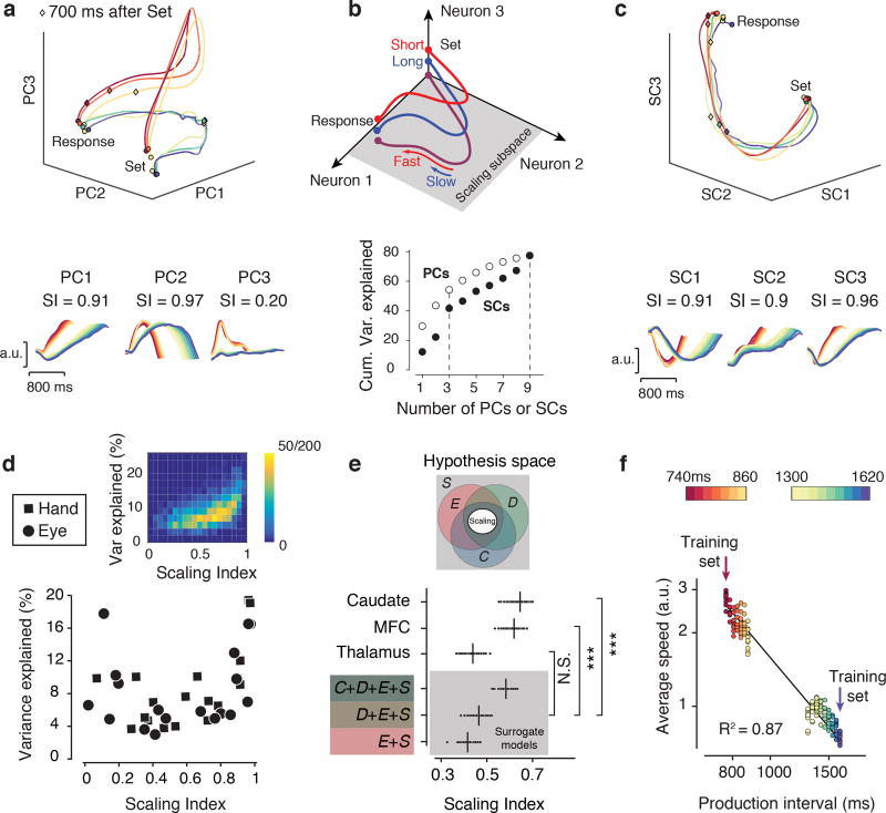
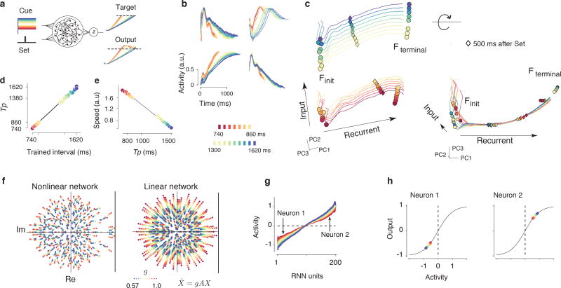
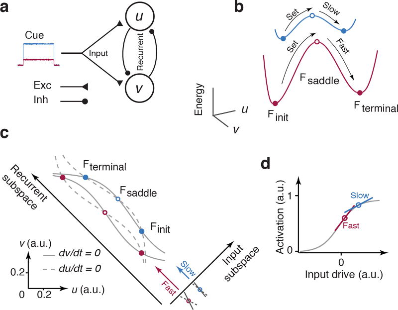
Musicians can perform at different tempos, speakers can control the cadence of their speech, and children can flexibly vary their temporal expectations of events. To understand the neural basis of such flexibility, we recorded from the medial frontal cortex of nonhuman primates trained to produce different time intervals with different effectors. Neural responses were heterogeneous, nonlinear, and complex, and they exhibited a remarkable form of temporal invariance: firing rate profiles were temporally scaled to match the produced intervals. Recording from downstream neurons in the caudate and from thalamic neurons projecting to the medial frontal cortex indicated that this phenomenon originates within cortical networks. Recurrent neural network models trained to perform the task revealed that temporal scaling emerges from nonlinearities in the network and that the degree of scaling is controlled by the strength of external input. These findings demonstrate a simple and general mechanism for conferring temporal flexibility upon sensorimotor and cognitive functions.

PubMed Disclaimer

Conflict of interest statement

Competing financial interests statement

The authors declare no conflicting interests.

Figures

Fig. 1

Fig. 1. Time production task and behavior

(a) Trial structure. Animals produced either an 800 ms (Short) or a 1500 ms (Long), either by making a saccade (Eye) or a button press (Hand). These four conditions were randomly interleaved and were cued throughout the trial by the color and shape of two central stimuli, a circular fixation for the eye and a square that cued the animal to place its hand on a button. The colored shape (circle or square) cued the effector, and the hue (red or blue) cued the desired interval (red for Short and blue for Long). After a random delay, a white circle was flashed to the left or right of the fixation point. This peripheral flash specified the saccadic target for the eye trials and played no role in the hand trials. After another random delay, a Set cue (a ring flashed around the fixation stimuli) initiated the motor timing epoch. The animal’s production interval (Tp) was measured as the interval between Set and when either the saccade was made or the button was pressed. When Tp was generated with the desired effector and was within a specified reward window, the peripheral target (or the square fixation) turned green, auditory feedback was provided, and animal received juice. The reward window was adjusted adaptively on a trial-by-trial basis and independently for the Short and Long conditions so that the animal received reward on approximately 50% of trials for both interval context on every session (on average, 57% in monkey A and 51% in monkey D). The reward magnitude increased linearly with accuracy as shown by the green triangular reward function. Two example trials, one for the Eye/Short (ES) condition (left) and one for the Hand/Long (HL) condition are shown. (b) A typical behavioral session showing Tp while the animal flexibly switched between the four trial conditions. For clarity the Eye (left) and Hand (right) trials are plotted separately although during the task they were randomly interleaved. The top 4 histograms show the distribution of Tp for each condition with rewarded trials in green. The vertical lines correspond to the mean values that are also reported numerically. (c) For both effectors (left: Eye, right: Hand) and both animals (top: animal A, bottom: animal D), the standard deviation of Tp scaled with mean Tp (red: Short, blue: Long). For animal A, the mean ± s.e.m of Tps across the conditions were ES: 810±48.9 ms, EL: 1495±117 ms, HS: 822.3±53.7 ms, HL: 1486±136 ms. For animal D, they were ES: 808±56.1 ms, EL: 1481±137 ms, HS: 836.7±91.3 ms HL: 1521±177 ms. The variability was significantly higher for the Long compared to the Short. The average Weber fraction (ratio of standard deviation to mean) for the Hand (β_Hand) was significantly larger that Eye (β_Eye) (one-tailed paired sample t-test, for monkey A, n = 31, t₃₀ = 1.80, P = .041, and for monkey D, n = 35, t₃₄ = 6.44, P < .001).

Fig. 2

Fig. 2. Medial frontal cortex inactivation and electrophysiology

(a) Parasagittal view of the brain of one animal (monkey D) with a red ellipse showing the targeted region. Stereotactic coordinates used in each animal are shown with respect to anterior commissure (AC) and midline (ML). (b) Muscimol inactivation. Each line in each panel shows the change in mean squared error (MSE = Σ(Tp − Ts)² = Bias² + Var) computed from mini-session (randomly sampled subsets of trials without replacement; see Methods) before and after the injection of muscimol (above) and saline (below) for the two intervals (red: Short, blue: Long) and two effectors (circle: Eye, square: Hand). The white-over-black bar graphs partition MSE to Bias (black) and Variance (white). Significance tests correspond to comparisons of MSE (see Table 1 for details) across mini-sessions (n: number of mini-sessions, **: P < .001, N.S.: not significant). (c) Average firing rates were computed after aligning spike times to movement initiation time. Top: Raster plot of spike times (black ticks) for an example neuron aligned to movement initiation time (dashed line) across trials (rows). Trials were sorted and grouped into bins according to the produced interval (Tp). Bottom: Average firing rates for each Tp bin plotted with respect to the time of Set (dashed line). The Set time in the top panel, and the activity profiles in the bottom panels were colored according to Tp bins (legend). (d) Activity profile of 8 example neurons for Hand (top) and Eye (bottom) conditions computed as described in (c). (e) Analysis of single neurons with respect to various model of timing (n = 416 neurons for both animals). Whisker plot showing the range of R² values captured by seven models fitted to the average firing rates of individual neurons (median: center line; box: 25th to 75th percentiles; whiskers: ×ばつ the interquartile range; dots: neurons whose R² values lie outside whiskers). The "Temporal scaling" model (top) had the highest explanatory power (R²) across models (one-way ANOVA, F_{6, 2859} = 125.2, P < .001, and one-tailed paired sample t-test between ‘Temporal scaling’ and ‘Population clock’ model, n = 416, t₄₁₅ = 6.32, ***P < .001). Models firs were cross-validated.

Fig. 3

Fig. 3. Temporal scaling in the medial frontal cortex at the population level

(a) Top: Population activity for Hand trials for Monkey A projected onto the first 3 principal components (PCs) from the time of Set to the time of button press (Response). Activity profiles associated with different produced intervals are plotted in different colors (see color bar in Fig. 3f). Diamond shows activity 700 ms after Set. Bottom: The time course of the first three PCs with the corresponding scaling index (SI) values. (b) Top: Schematic drawing illustrating the scaling subspace. The response dynamics associated with Short (red) and Long (blue) produced interval (Tp) are depicted as distinct trajectories in the state space. Projections of neural responses onto a scaling subspace result in overlapping trajectories (purple) whose speed determines the produced interval, fast for Short (red) and slow for Long (blue). Bottom: Cumulative percentage variance explained by PCs and scaling components (SCs). (c) Top: Population activity sorted according to Tp bins and projected onto the first 3 SCs. As expected, in this subspace, the trajectories overlap. Bottom: The first three SCs with the corresponding SI values. Because of cross-validation, SIs were not in decreasing order (see text). (d) Variance explained for individual SCs as a function of SI. SCs with the larger SI explain a large percentage of variance for both Hand (square) and Eye (circle) conditions. Inset: Variance explained as a function of SI derived along 200 random one-dimensional projections of MFC activity in the state space. Individual projections were binned and pseudocolored to indicate the frequency of occurrence. The data shows that high scaling indices are associated with high variance explained. (e) Comparison of SI in the MFC, caudate and thalamus with surrogate data generated from three Gaussian process models that were constrained to match the observed response profiles with increasing levels of sophistication (Supplementary Note and Supplementary Fig. 3). The inset shows the hypothesis space in relation to various constraints and their combinations with distinct colors and their overlaps. Perfect scaling (middle ellipse) is a subset of the possibilities that satisfy all four constraints. Each model consisted of the same number of neurons as that in the MFC data, and the number of bootstrapped samples for each model was n = 200. The plot shows the the average SI across all SCs computed from bootstraps (small circles) along with the corresponding mean (vertical line) for each of three brain areas and each of the surrogate models. The average SI for each surrogate model was significantly lower than the values associated with the MFC and caudate, but not for the thalamus (see main text for statistics). (f) The speed of neural trajectory within the scaling subspace spanned by the first 3 SCs predicted average Tps across bins. The relationship between speed and Tp was fit to a linear log-log function. The scaling subspace was computed from training data (arrows, 2 Tp bins) and used to evaluate speed on the remaining test data (14 Tp bins). R² was computed by repeating the procedure using bootstrapping (n = 10). Both axes are in log scale.

Fig. 4

Fig. 4. Inactivation, electrophysiology and temporal scaling in the caudate and thalamus

(a) Same as Fig. 2a with a red ellipse and stereotactic coordinates showing targeted regions in the caudate. (b) Muscimol inactivation in the caudate. Results are presented in the same format as in Fig. 2b. (c) Activity profile of three example caudate neurons (same format as in Fig. 2d). (d) Top: The relationship between variance explained and scaling index (SI) in the caudate (same format as the inset of Fig. 3d). Bottom: The first three PCs with the corresponding SI values. (e) Same as panel a showing the region of interest in the thalamus. We recorded from neurons in the region where MFC-projecting neurons were identified antidromically. Inset: example of reliable and low-latency spikes detected after antidromic stimulation. (f–h) Inactivation, electrophysiology and temporal scaling in the thalamus (same format as panels b–d). Responses in the thalamus are qualitatively different from the caudate (panel d) and MFC (Fig. 3d) in that most projections in the state space do not exhibit temporal scaling.

Fig. 5

Fig. 5. Recurrent neural network model dynamics

(a) A recurrent neural network model that receives an input (Cue) whose strength depends on the desired interval (different colors), and a transient Set pulse that initiates the timing interval. The model produces a "response" when its output (z) reaches a fixed threshold. Network was trained to produce a linear ramp at its output. For other objectives see Supplementary Fig. 6. (b) The response profiles of randomly selected units aligned to the time of Set. Many units exhibit temporal scaling. (c) Left: Network activity projected onto the first three principal components (PCs) across all trials. Different traces correspond to trials with different durations (red for shortest to blue for longest). For each Cue input, the network engenders an initial and a terminal fixed point (circles; F_init and F_terminal). Diamonds mark the state of the network along the trajectory 500 ms after Set. The Cue input moves the fixed points within an "Input" subspace. The corresponding trajectories for different intervals reside in a separate "Recurrent" subspace. Right: Rotation of the state space reveals the invariance of trajectories in the recurrent subspace. In the recurrent subspace trajectories traverse the same path at different speeds (see diamonds for different Cue inputs). (d) After training, the network accurately produced the intervals according to the presented Cue input. (e) A plot of the average speed in the recurrent neural network model as a function of the production interval (Tp) on a log-log scale. The speed was estimated from the rate of change of activity along the neural trajectory within the subspace spanned by the first three PCs. (f) Left: The spectrum of eigenvalues of the linearized dynamics near F_terminal. Right: The spectrum of eigenvalues of an N-dimensional linear dynamical system τẋ = gAx, with elements of A sampled from a Normal distribution N(0,1 / N). Decreasing the gain values from g = 1.0 (red) to 0.57 (blue) progressively decreases the magnitude of the eigenvalues and increases the effective time constants τ_eff = τ / g. (g) Units in recurrent model were sorted based on their maximal activity when the network was near F_terminal. The plot shows the maximum activity as function of Cue input. Vertical arrows mark two neurons, one with positive and another with negative activity, which are plotted in panel (h). (h) Stronger input drives units toward the saturation point of their nonlinear activation function where the shallowness of slopes leads to reduced gain of neural activity. This is true both for units with a positive response whose responses increased with Cue input (right), as well as units with a negative response, whose responses decreased with input drive (left). In all plots, different colors correspond to different intervals as shown by the color bar.

Figure 6

Figure 6. A simple two-neuron implementation of speed control

(a) Two inhibitory units (u and v) with recurrent inhibition receive a common excitatory input (Cue). (b) The energy landscape of the two-neuron model. The network has a bistable energy landscape whose gradients depend on the strength of the Cue input. Stronger inputs (blue) lead to shallower energy gradients and vice versa (red). The Set pulse moves the state away from the initial fixed point (F_init, filled circle) and over the saddle point (F_saddle, open circle). The network then spontaneously moves toward the terminal fixed point (F_terminal, filled circle). The speed of the movement toward F_terminal is relatively slow when the energy gradient is shallow (blue) due to stronger common input. (c) Phase plane analysis of the 2-neuron model. The two axes on the lower left correspond to the activity of the two neurons (u and v). The input is applied to both units and thus drives the system along the diagonal, labeled as "input subspace". The input level moves the sigmoidal nullclines of the two units (du/dt = 0, dashed, and dv/dt = 0, solid, see Supplementary Note) and adjusts the location of the three fixed points (F_init, F_terminal and the intermediate F_saddle). The figure shows the two nullclines and the corresponding fixed points for two inputs levels (red and blue). Activation of Set moves the system along a "recurrent subspace" which is orthogonal to the input subspace. The proximity of nullclines (crosses below the Input subspace) controls the speed. When the input is stronger, the nullclines are closer, which causes the system to become slower. (d) Interaction of the input drive with the saturating nonlinearity of one unit. The action of the input upon the nonlinear activation functions moves the saddle point and controls the speed of the system. Stronger inputs push the neurons toward the shallower part of the nonlinear activation function, and moves the saddle point to slower regions of the phase plane causing recurrent interactions to slow down.

See this image and copyright information in PMC

References

1. Stuphorn V, Schall JD. Executive control of countermanding saccades by the supplementary eye field. Nat. Neurosci. 2006;9:925–931. - PubMed
1. Kunimatsu J, Tanaka M. Alteration of the timing of self-initiated but not reactive saccades by electrical stimulation in the supplementary eye field. Eur. J. Neurosci. 2012;36:3258–3268. - PubMed
1. Fried I, et al. Functional organization of human supplementary motor cortex studied by electrical stimulation. J. Neurosci. 1991;11:3656–3666. - PMC - PubMed
1. Lewis PA, Wing AM, Pope PA, Praamstra P, Miall RC. Brain activity correlates differentially with increasing temporal complexity of rhythms during initialisation, synchronisation, and continuation phases of paced finger tapping. Neuropsychologia. 2004;42:1301–1312. - PubMed
1. Shima K, Tanji J. Neuronal activity in the supplementary and presupplementary motor areas for temporal organization of multiple movements. J. Neurophysiol. 2000;84:2148–2160. - PubMed

Publication types

Actions
Actions

MeSH terms

Actions
Actions
Actions
Actions
Actions
Actions
Actions
Actions
Actions
Actions
Actions
Actions
Actions
Actions
Actions
Actions
Actions
Actions

Substances

Actions
Actions

Grants and funding

R01 NS078127/NS/NINDS NIH HHS/United States

LinkOut - more resources

Full Text Sources
Other Literature Sources
- scite Smart Citations

[1] Stuphorn V, Schall JD. Executive control of countermanding saccades by the supplementary eye field. Nat. Neurosci. 2006;9:925–931. - PubMed

[2] Stuphorn V, Schall JD. Executive control of countermanding saccades by the supplementary eye field. Nat. Neurosci. 2006;9:925–931. - PubMed

[3] Kunimatsu J, Tanaka M. Alteration of the timing of self-initiated but not reactive saccades by electrical stimulation in the supplementary eye field. Eur. J. Neurosci. 2012;36:3258–3268. - PubMed

[4] Kunimatsu J, Tanaka M. Alteration of the timing of self-initiated but not reactive saccades by electrical stimulation in the supplementary eye field. Eur. J. Neurosci. 2012;36:3258–3268. - PubMed

[5] Fried I, et al. Functional organization of human supplementary motor cortex studied by electrical stimulation. J. Neurosci. 1991;11:3656–3666. - PMC - PubMed

[6] Fried I, et al. Functional organization of human supplementary motor cortex studied by electrical stimulation. J. Neurosci. 1991;11:3656–3666. - PMC - PubMed

[7] Lewis PA, Wing AM, Pope PA, Praamstra P, Miall RC. Brain activity correlates differentially with increasing temporal complexity of rhythms during initialisation, synchronisation, and continuation phases of paced finger tapping. Neuropsychologia. 2004;42:1301–1312. - PubMed

[8] Lewis PA, Wing AM, Pope PA, Praamstra P, Miall RC. Brain activity correlates differentially with increasing temporal complexity of rhythms during initialisation, synchronisation, and continuation phases of paced finger tapping. Neuropsychologia. 2004;42:1301–1312. - PubMed

[9] Shima K, Tanji J. Neuronal activity in the supplementary and presupplementary motor areas for temporal organization of multiple movements. J. Neurophysiol. 2000;84:2148–2160. - PubMed

[10] Shima K, Tanji J. Neuronal activity in the supplementary and presupplementary motor areas for temporal organization of multiple movements. J. Neurophysiol. 2000;84:2148–2160. - PubMed

Account

Save citation to file

Email citation

Add to Collections

Add to My Bibliography

Your saved search

Create a file for external citation management software

Your RSS Feed

Flexible timing by temporal scaling of cortical responses

Affiliations

Flexible timing by temporal scaling of cortical responses

Authors

Affiliations

Abstract

Conflict of interest statement

Figures

References

Publication types

MeSH terms

Substances

Grants and funding

LinkOut - more resources

Full Text Sources

Other Literature Sources